SOURCE FOR CONTENT:
Priest, E. Magnetohydrodynamics of the Sun, 2014. Cambridge University Press. Ch.2.;
Davidson, P.A., 2001. An Introduction to Magnetohydrodynamics. Ch.4.
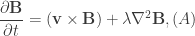
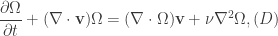
We have seen how to derive the induction equation from Maxwell’s equations assuming no charge and assuming that the plasma velocity is non-relativistic. Thus, we have the induction equation as being

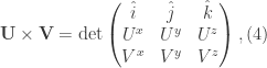
Many texts in MHD make the comparison of the induction equation to the vorticity equation

where I have made use of the vector identity
 .
.
Indeed, if we do compare the induction equation (Eq.(1)) to the vorticity equation (Eq.(2)) we easily see the resemblance between the two. The first term on the right hand side of Eq.(1)/ Eq.(2) determines the advection of magnetic field lines/vortex field lines; the second term on the right hand side deals with the diffusion of the magnetic field lines/vortex field lines.
From this, we can impose restrictions and thus look at the consequences of the induction equation (since it governs the evolution of the magnetic field). Furthermore, we see that we can modify the kinematic theorems of classical vortex dynamics to describe the properties of magnetic field lines. After discussing the direct consequences of the induction equation, I will discuss a few theorems of vortex dynamics and then introduce their MHD analogue.
Inherent to this is magnetic Reynold’s number. In geophysical fluid dynamics, the Reynolds number (not the magnetic Reynolds number) is a ratio between the viscous forces per volume and the inertial forces per volume given by

where  represent the typical fluid velocity, length scale and typical volume respectively. The magnetic Reynolds number is the ratio between the advective and diffusive terms of the induction equation. There are two canoncial regimes: (1)
  , and (2)
 The former is sometimes called the diffusive limit and the latter is called either the Ideal limit or the infinite conductivity limit (I prefer to call it the ideal limit, since the terms infinite conductivity limit is not quite accurate).
Case I:
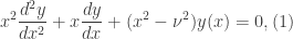
Consider again the induction equation

If we then assume that we are dealing with incompressible flows (i.e.  ) then we can use the aforementioned vector identity to write the induction equation as

In the regime for which , the induction equation for incompressible flows (Eq.(4)) assumes the form
Compare this now to the following equation,
We see that the magnetic field lines are diffused through the plasma.
Case II:
If we now consider the case for which the advective term dominates, we see that the induction equation takes the form

Mathematically, what this suggests is that the magnetic field lines become “frozen-in” the plasma, giving rise to Alfven’s theorem of flux freezing.
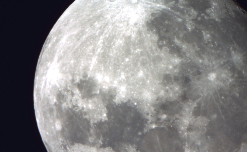
Many astrophysical systems require a high magnetic Reynolds number. Such systems include the solar magnetic field (heliospheric current sheet), planetary dynamos (Earth, Jupiter, and Saturn), and galactic magnetic fields.
Kelvin’s Theorem & Helmholtz’s Theorem:
Kelvin’s Theorem: Consider a vortex tube in which we have that  , in which case

and consider also the curve taken around a closed surface, (we call this curve a material curve  ) we may define the circulation as being
Thus, Kelvin’s theorem states that if the material curve is closed and it consists of identical fluid particles then the circulation, given by Eq.(9), is temporally invariant.
Helmholtz’s Theorem:
Part I: Suppose we consider a fluid element which lies on a vortex line at some initial time  , according to this theorem it states that this fluid element will continue to lie on that vortex line indefinitely.
Part II: This part says that the flux of vorticity

remains constant for each cross-sectional area and is also invariant with respect to time.
Now the magnetic analogue of Helmholtz’s Theorems are found to be Alfven’s theorem of flux freezing and conservation of magnetic flux, magnetic field lines, and magnetic topology.
The first says that fluid elements which lie along magnetic field lines will continue to do so indefinitely; basically the same for the first Helmholtz theorem.
The second requires a more detailed argument to demonstrate why it works but it says that the magnetic flux through the plasma remains constant. The third says that magnetic field lines, hence the magnetic structure may be stretched and deformed in many ways, but the magnetic topology overall remains the same.
The justification for these last two require some proof-like arguments and I will leave that to another post.
In my project, I considered the case of high magnetic Reynolds number in order to examine the MHD processes present in region of metallic hydrogen present in Jupiter’s interior.
In the next post, I will “prove” the theorems I mention and discuss the project.


![\displaystyle a_{0}\bigg\{r(r-1)+r\bigg\}x^{r}+a_{1}\bigg\{(1+r)r+(1+r)\bigg\}x^{r+1}+\sum_{j=2}^{\infty}\bigg\{[(j+r)(j+r-1)+(j+r)]a_{j}+a_{j-2}\bigg\}x^{j+r}=0, (7)](https://s0.wp.com/latex.php?latex=%5Cdisplaystyle+a_%7B0%7D%5Cbigg%5C%7Br%28r-1%29%2Br%5Cbigg%5C%7Dx%5E%7Br%7D%2Ba_%7B1%7D%5Cbigg%5C%7B%281%2Br%29r%2B%281%2Br%29%5Cbigg%5C%7Dx%5E%7Br%2B1%7D%2B%5Csum_%7Bj%3D2%7D%5E%7B%5Cinfty%7D%5Cbigg%5C%7B%5B%28j%2Br%29%28j%2Br-1%29%2B%28j%2Br%29%5Da_%7Bj%7D%2Ba_%7Bj-2%7D%5Cbigg%5C%7Dx%5E%7Bj%2Br%7D%3D0%2C+%287%29&bg=ffffff&fg=333333&s=0&c=20201002)


![\displaystyle a_{j}(r)=\frac{-a_{j-2}(r)}{[(j+r)(j+r-1)+(j+r)]}=\frac{-a_{j-2}(r)}{(j+r)^{2}}. (9)](https://s0.wp.com/latex.php?latex=%5Cdisplaystyle+a_%7Bj%7D%28r%29%3D%5Cfrac%7B-a_%7Bj-2%7D%28r%29%7D%7B%5B%28j%2Br%29%28j%2Br-1%29%2B%28j%2Br%29%5D%7D%3D%5Cfrac%7B-a_%7Bj-2%7D%28r%29%7D%7B%28j%2Br%29%5E%7B2%7D%7D.+%289%29&bg=ffffff&fg=333333&s=0&c=20201002)


 , then the conjugate vector takes the form

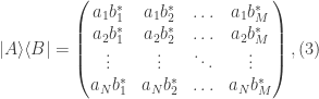


 . Therefore we can write any arbitrary vector in the following way

 represent the outer product which may also be written in component form as
  . We therefore have the condition that

 . The first relation represents the completeness of an orthonormal set of basis vectors and the second is its modified form.
 as
as
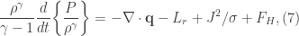
 represents the net effect of energy sinks and sources and is called the energy loss function. For simplicity, one typically writes the form of the heat equation to be
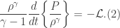
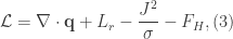
 represents heat flux by particle conduction,
  is the net radiation,
  is the Ohmic dissipation, and
  represents external heating sources, if any exist. The term
 is the thermal conduction tensor.


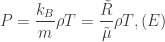 (Ideal Gas Law)
 (i.e. non-relativistic). Finally for incompressible flows we know that
 undefined. The second case will consider in a future post
  , where

 and using this and its variants we arrive at
![\displaystyle \sum_{j=0}^{\infty}[(j+2)(j+1)a_{j+2}-2ja_{j}+\lambda a_{j}]x^{j}=0. (7)](https://s0.wp.com/latex.php?latex=%5Cdisplaystyle+%5Csum_%7Bj%3D0%7D%5E%7B%5Cinfty%7D%5B%28j%2B2%29%28j%2B1%29a_%7Bj%2B2%7D-2ja_%7Bj%7D%2B%5Clambda+a_%7Bj%7D%5Dx%5E%7Bj%7D%3D0.+%287%29&bg=ffffff&fg=333333&s=0&c=20201002)
 , we therefore require that

 we arrive at two linearly independent solutions (one even and one odd) in terms of the fundamental coefficients
  and
and  which may be written as
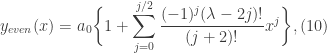


 ,
,
 and
and  corresponding to the even and odd expressions for the Legendre polynomials.
 and angles
  . The law of cosines therefore maintains that
 from the left hand side of Eq.(1), take the square root and invert this yielding
 , therefore the binomial expansion is
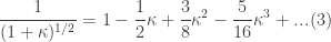
 we get
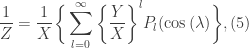
![\displaystyle \frac{1}{Z}=\frac{1}{\sqrt[]{X^{2}+Y^{2}-2XY\cos{(\lambda)}}}=\sum_{l=0}^{\infty}\frac{Y^{l}}{X^{l+1}}P_{l}(\cos{(\lambda)}. (6)](https://s0.wp.com/latex.php?latex=%5Cdisplaystyle+%5Cfrac%7B1%7D%7BZ%7D%3D%5Cfrac%7B1%7D%7B%5Csqrt%5B%5D%7BX%5E%7B2%7D%2BY%5E%7B2%7D-2XY%5Ccos%7B%28%5Clambda%29%7D%7D%7D%3D%5Csum_%7Bl%3D0%7D%5E%7B%5Cinfty%7D%5Cfrac%7BY%5E%7Bl%7D%7D%7BX%5E%7Bl%2B1%7D%7DP_%7Bl%7D%28%5Ccos%7B%28%5Clambda%29%7D.+%286%29&bg=ffffff&fg=333333&s=0&c=20201002)
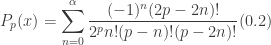
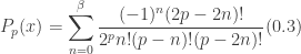
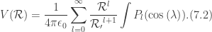
 generates the Legendre polynomials. Two prominent uses of these polynomials includes gravity and its application to the theory of potentials of a spherical mass distributions, and the other is that of electrostatics. For example, suppose we have the potential equation
 associated with a point P are said to be components of a second-order tensor if, under a change of coordinates, from a set of coordinates
  to
to  , they transform according to
 ,etc. If we consider further more and more vectors, we can therefore imagine a space constituted by these vectors; a vector space. To make it formal, here is the definition:
 is the nonempty set of elements (vectors) that satisfy the following axioms


 , and
, and  is a scalar, then
  .
. , then
  .
. in the following manner


 denotes the Kronecker delta:

 -th component is
 denotes the Levi-Civita symbol. If these indices form an odd permutation
  , if the indices form an even permutation
  , and if any of these indices are equal
  .
. , they collectively describe what is referred to as an event. Formally, an event in spacetime is described by three spatial coordinates and one time coordinate. We may replace these coordinates by
  , where
  in which I am defining
  . In words, this means that the index
  is an integer that is greater than or equal to 0.
 corresponds to time,
  correspond to the x,y, and z coordinates respectively. Therefore,
  is called the four-position.

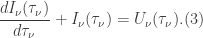
 and
and  are the emission and absorption coefficients, respectively. We can further define the absorption coefficient to be equivalent to
  . Hence,
 yielding
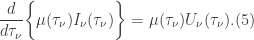
 . To show that this is valid, consider the equation for
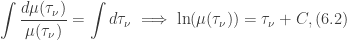
 is some constant of integration. Let us assume that the constant of integration is
  , and let us also take the exponential of (6.2). This gives us
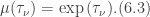
 ,
,
 , hence we have that
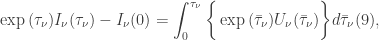
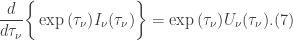
 and divide by
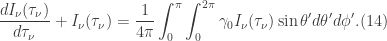
  we arrive at the general solution of the radiative transfer equation
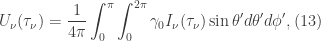
 -th approximation for isotropic scattering).
 via the following
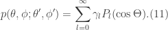
 in the sum given by (11). This then would mean that the phase function is constant
 we find that this force is proportional to Hooke’s law of elasticity, that is,
  . If we consider other forces we also find that there exists a force balance between the restoring force (our applied force), a resistance force, and a forcing function, which we assume to have the form
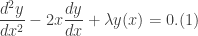
 . Therefore, we actually have a system of three second order linear non-homogeneous ordinary differential equations in three variables:


 ,
,  , and
, and  . Furthermore, I am only going to consider the
  component of this system. Thus, the equation that we seek to solve is

 is the particular solution to the non-homogeneous equation and the other two terms are the fundamental solutions of the homogeneous equation:
 . Taking the first and second time derivatives, we get
  and
and  . Therefore, Eq. (6) becomes, after factoring out the exponential term,
![D\exp{(\lambda t)}[\lambda^{2}+\gamma \lambda +\omega_{0}]=0. (7)](https://s0.wp.com/latex.php?latex=D%5Cexp%7B%28%5Clambda+t%29%7D%5B%5Clambda%5E%7B2%7D%2B%5Cgamma+%5Clambda+%2B%5Comega_%7B0%7D%5D%3D0.%C2%A0+%287%29&bg=ffffff&fg=333333&s=0&c=20201002)
 , it follows that
![\lambda =\frac{-\gamma \pm \sqrt[]{\gamma^{2}-4\omega_{0}}}{2}. (9)](https://s0.wp.com/latex.php?latex=%5Clambda+%3D%5Cfrac%7B-%5Cgamma+%5Cpm+%5Csqrt%5B%5D%7B%5Cgamma%5E%7B2%7D-4%5Comega_%7B0%7D%7D%7D%7B2%7D.+%289%29&bg=ffffff&fg=333333&s=0&c=20201002)
![\sqrt[]{\gamma^{2}-4\omega_{0}}](https://s0.wp.com/latex.php?latex=%5Csqrt%5B%5D%7B%5Cgamma%5E%7B2%7D-4%5Comega_%7B0%7D%7D&bg=ffffff&fg=333333&s=0&c=20201002) is greater than, equal to , or less than 0, and the consequent solutions. I will also obtain the solution to the non-homogeneous equation in that post as well.
is greater than, equal to , or less than 0, and the consequent solutions. I will also obtain the solution to the non-homogeneous equation in that post as well.