SOURCES FOR CONTENT:
- Chandrasekhar, S., 1960. “Radiative Transfer”. Dover. 1.
- Choudhuri, A.R., 2010. “Astrophysics for Physicists”. Cambridge University Press. 2.
- Boyce, W.E., and DiPrima, R.C., 2005. “Elementary Differential Equations”. John Wiley & Sons. 2.1.
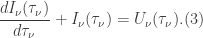
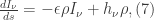
Recall from last time , the radiative transfer equation

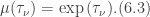
where 


which upon rearrangement and substitution in Eq. (1) gives
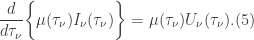
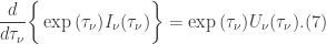
We may solve this equation by using the method of integrating factors, by which we multiply Eq.(3) by some unknown function (the integrating factor) 

Upon examining Eq.(4), we see that the left hand side is the product rule. It follows that
This only works if 

This is a separable ordinary differential equation so we can rearrange and integrate to get
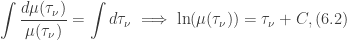
where 

This is our integrating factor. Just as a check, let us take the derivative of our integrating factor with respect to 

Thus this requirement is satisfied. If we now return to Eq.(4) and substitute in our integrating factor we get
We can treat this as a separable differential equation so we can integrate immediately. However, we are integrating from an optical depth 

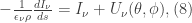
We find that
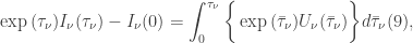
where if we add 


This is the mathematically formal solution to the radiative transfer equation. While mathematically sound, much of the more interesting physical phenomena require more complicated equations and therefore more sophisticated methods of solving them (an example would be the use of quadrature formulae or 
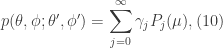
Recall also that in general we can write the phase function 
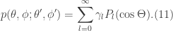
Let us consider the case for which 

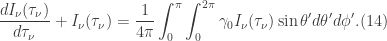
Such a phase function is consistent with isotropic scattering. The term isotropic means, in this context, that radiation scattered is the same in all directions. Such a case yields a source function of the form
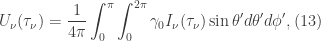
where upon use in the radiative transfer equation we get the integro-differential equation
Solution of this equation is beyond the scope of the project. In the next post I will discuss Rayleigh scattering and the corresponding phase function.
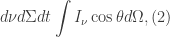
 passing through an area
  constrained to a solid angle
  in a time
  . We may write this mathematically as
 we get
 be an element of the surface
  in a volume
  through which radiation passes. Further let
  and
and  denote the angles which form normals with respect to elements
  . These surfaces are joined by these normals and hence we have the surface across which energy flows includes the elements
 is the solid angle subtended by the surface element
  and volume element
  is the volume that is intercepted in volume
 in the volume, then we must multiply Eq.(5) by
  , where
  is the speed of light.

 represents the source function given by
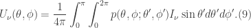
 (in keeping with our notation in
