Basics of Tensor Calculus and General Relativity-Vectors and Introduction to Tensors (Part II-Continuation of Vectors)

SOURCE FOR CONTENT: Neuenschwander, D.E., 2015. Tensor Calculus for Physics. Johns Hopkins University Press. Ch.1

In the preceding post of this series, we saw how we may define a vector in the traditional sense. There is another formulation which is the focus of this post. One becomes familiar with this formulation typically in a second course in quantum mechanics or of a similar form in an introductory linear algebra course.

A vector may be written in two forms: a ket vector,

$\displaystyle |A\rangle=\begin{pmatrix} a_{1}&\\ a_{2}&\\ \vdots &\\ a_{N} \end{pmatrix}, (1.1)$

or a bra vector (conjugate vector):

$\displaystyle \langle A|=\begin{pmatrix} a_{1} & a_{2} & \hdots & a_{N} \end{pmatrix}, (1.2)$

Additionally, if $\langle A| \in \mathbb{C}$ , then the conjugate vector takes the form

$\displaystyle \langle A|=\begin{pmatrix} a_{1}^{*} & a_{2}^{*} & \hdots & a_{N}^{*} \end{pmatrix}. (1.3)$

In words, if the conjugate vector exists in the complex plane, we may express such a vector in terms of complex conjugates of the components.

We may form the inner product by the following

$\displaystyle \langle A|B\rangle = a_{1}^{*}b_{1}+a_{2}^{*}b_{2}+\hdots+a_{N}^{*}b_{M}=\sum_{i=1}^{N}\sum_{j=1}^{M}a_{i}^{*}b_{j}. (2)$

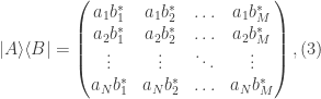
Conversely we may form the outer product as follows

$\displaystyle |A\rangle \langle B|= \begin{pmatrix} a_{1}b_{1}^{*} & a_{1}b_{2}^{*} & \hdots & a_{1}b_{M}^{*}\\ a_{2}b_{1}^{*} & a_{2}b_{2}^{*} & \hdots & a_{2}b_{M}^{*}\\ \vdots & \vdots & \ddots & \vdots \\ a_{N}b_{1}^{*} & a_{N}b_{2}^{*}& \hdots & a_{N}b_{M}^{*}\\ \end{pmatrix}, (3)$

Additionally, one typically defines a vector as a linear combination of basis vectors which we shall express by the following:

$\displaystyle \hat{i}=|1\rangle \equiv \begin{pmatrix} 1 \\ 0 \\ 0 \\ \end{pmatrix},$

$\displaystyle \hat{j} = |2\rangle \equiv \begin{pmatrix} 0 \\ 1 \\ 0 \\ \end{pmatrix},$

$\displaystyle \hat{k}=|3\rangle \equiv \begin{pmatrix} 0 \\ 0 \\ 1 \\ \end{pmatrix},$

where in general the basis vectors satisfy $\langle i|j \rangle = \delta_{ij}$ . Therefore we can write any arbitrary vector in the following way

$\displaystyle \textbf{A}= a_{1}|1\rangle + a_{2}|2\rangle + ... + a_{n}|n\rangle. (4)$

Moreover, any conjugate vector may be written as

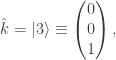
$\displaystyle \langle B|= b_{1}\langle 1| + b_{2}\langle 2| + ... + b_{m}\langle m|. (5)$

Let $\mathcal{P} = |A\rangle \langle B|$ represent the outer product which may also be written in component form as $\mathcal{P}_{ij}=\langle i|\mathcal{P}|j\rangle$ . We therefore have the condition that

$\displaystyle \textbf{1} = \sum_{\mu}|\mu\rangle \langle \mu|, (6)$

and

$\displaystyle |A\rangle = \sum_{\mu}|\mu\rangle \langle \mu|A\rangle =\sum_{\mu}A^{\mu}|\mu\rangle, (7)$

wherein $\displaystyle A^{\mu}\equiv \langle \mu|A\rangle$ . The first relation represents the completeness of an orthonormal set of basis vectors and the second is its modified form.

The next post will discuss the transformations of coordinates of vectors using both the matrix formulation and using partial derivatives.

Share this:

Like this:

Related

Leave a Reply Cancel reply