Real Analysis/Topology – Understanding Physics and Astronomy

A Very Brief Introduction to Measure Theory and the Lebesgue Integral (Part I)

In the next few posts, I shall be discussing recent topics of study that, to me at least, have been very intruiging. In previous posts, I have talked about Hilbert spaces. I have of late been considering the mathematics necessary to formally understand in a pure mathematical sense what a Hilbert space is. This post, like the others on this site, serves as a reference of newly learned topics that are of interest (to me, at least; such a comment is subjective, of course).

The purpose of this post is two-fold: (1.) to provide an update with what I’ve been up to; (2.) introduce some interesting mathematics that have expanded my understanding to the “size” of a set as well as operations such as differentiation and integration.

Here is a quick summary of what I plan to cover in the next few posts (to a brief extent):

Elementary Sets and their Measure: Here I will discuss the concept of length and try extend length in greater dimensions to that of a measure of a set. Much of this topic will rely on geometric intuition.
Lebesgue Measure: This section will dicuss the concept of Lebesgue measure and distinguish it from the elementary measure. Also brief mention will be made of measurability of sets and functions.
General Measure: Discussion will be made of a general measure as a function as well as measurable spaces and measure spaces.
Lebesgue Integral: This topic will introduce the concept of the Lebesgue integral as compared to the Riemann integral.
$L^{p}$ and $l^{p}$ spaces: This section will discuss the concept of a norm as it relates to the spaces $L^{p}$ and $l^{p}$ , and will define each space. We will also introduce the concept of Banach spaces.
Proof that $l^{p}$ space is a Banach space.

Section 1: Elementary Sets and their Measure:

The question that we want to answer is this: Given an arbitrary set, how do we go about measuring it?

In order to understand the difficulties present in this question we must first consider what are called elementary sets and the elementary measure. Elementary sets are those sets which are intuitively easy to measure; that is, intervals, rectangles, and boxes. We now give the formal definition of an elementary set:

Definition. (Interval; Elementary Set) We define an interval to be a subset of the real line $\mathbb{R}$ which take one of the following forms:

$[a,b] := \{x\in \mathbb{R}|a\leq x \leq b\} \label{(1.1)}$ ;

$[a,b) := \{x\in \mathbb{R}|a\leq x < b\} \label{(1.2)}$ ;

$(a,b] := \{x\in \mathbb{R}|a< x\leq b\} \label{(1.3)}$ ;

$(a,b):= \{x\in \mathbb{R}|a< x< b\} \label{(1.4)}$ ,

The length of an interval $I=[a,b]$ denoted $l(I):= b-a$ . For dimensions $d\geq 2$ , we define the measure of such sets as equalling the $d$ -times Cartesian product of intervals $I_{d}$ ; that is,

$\displaystyle m(B) := \prod_{i=1}^{d}l(I_{i}); \label{(2)}$

we sometimes call sets of dimension 2 or greater as “boxes.” Thus, elementary sets are those subsets of $\mathbb{R}^{d}$ such that

$\displaystyle m(E)= \bigcup_{i=1}^{d}m(B_{i}), \label{(3)}$

where $B$ is $i$ -th $d$ -dimensional box contained in $\mathbb{R}^{d}$ .

What this definition is doing is the following: first it introduces the concept of an interval and establishes the well-understood concept of its length as being the difference between the two endpoints provided one is less than the other. The definition then generalizes the idea of a length to 2 and 3 dimensions and beyond. Note that in 2-dimensions the interval then becomes a rectangle in the plane. Thus, the measure of the length of an interval then becomes the measure of the area of a rectangle. Similarly, for $d=3$ we replace rectangles with cubes and the area with the volume. For dimensions $d>3$ , we replace cubes with boxes of $d$ -dimension. Therefore, elementary sets are those subsets of $d$ -dimensional real space that are unions of finitely-many boxes.

Section 2: Lebesgue Measure

In the last section, we discussed sets for which we can measure quite easily. Though ideally we would like to be able to measure more general sets; that is, sets that are more general than elementary sets. Therefore, we require a different way of measurement. Thus, we come to need the Lebesgue measure.

In order to introduce the Lebesgue measure we need to first introduce the concept of the outer measure, which we now define

Definition. (Outer Measure) We define the outer measure of a set $E\subset \mathbb{R}$ , denoted $m^{*}(E)$ to be

$\displaystyle m^{*}(E) = \inf\bigg\{\sum_{k=1}^{\infty}l(I_{k})|\forall k\in \mathbb{N}, I_{k} \text{ is open such that } E \subset \bigcup_{k=1}^{\infty}I_{k}\bigg\}.$

The outer measure of a set in a sense “overestimates” the size of a given set and then takes the smallest such overestimate to within a specified tolerance. Thus, it estimates the size of the given set “from the outside,” and is used in lieu of the elementary measure when we are dealing with sets that we cannot easily measure the set in a geometrically-intuitive way.

We conclude this post with the definition of the Lebesgue measure given in two forms; the first will be in terms of what we have defined so far, and the second will be defined in terms that will be covered in the next post.

Definition. (Lebesgue Measure.) We define the Lebesgue measure of the set $E$ to be a set whose measure $m(E)=m^{*}(E)$ ; that is, its measure is equal to the outer measure.

The second way of defining this is as follows:

Definition. (Lebesgue Measure V.2) The Lebesgue measure is the measure on the measureable space $(\mathbb{R},\mathcal{L})$ where $\mathcal{L}$ is the $\sigma$ -algebra of Lebesgue measurable subsets of $\mathbb{R}$ that assigns to each Lebesgue measurable set its outer measure.

The next post will discuss measures in general, as well as measurable sets, measureable spaces, Borel sets, and $\sigma$ -algebras.

Until then, clear skies!

Open covers, Finite Subcovers, and COMPACTNESS

A second topological concept that is introduced in analysis is compactness. It is a concept that is associated with the Bolzano-Weierstrass Theorem which is as follows

THM. (Bolzano-Weierstrass). Let $A$ be any infinite bounded set of $\mathbb{R}$ . Then there is at least one $x\in \mathbb{R}$ such that every open ball centered on $x$ will contain at least one point in $A$ .

The idea of the proof of this statement is to show that the intersection $B_{x}(\epsilon)\cap A \neq \emptyset$ .

Insofar as compactness is concerned, there are a few different ways to introduce the concept. I will present the various definitions and show that they are all equivalent.

Method 1: Open Covers and Finite Subcovers.
In order to define compactness in this way, we need to define a few things; the first of which is an open cover.

Definition. [Open Cover.] Let $(X,d)$ be a metric space with the defined metric $d$ . Let $A\subset (X,d)$ . Then an open cover for $A$ is a collection of open sets $\{O_{\alpha}|\alpha \in \mathbb{N}\}$ such that
$\displaystyle A \subset \bigcup_{\alpha\in \mathbb{N}}O_{\alpha}$ .

N.B. The collection of open subsets $O_{\alpha}$ may be of infinite cardinality.

Another definition that we will need is the following:

Definition. [Limit Point/Cluster Point.] Let $(X,d)$ be a metric space and let $B\subset (X,d)$ , and let $x_{0}\in X$ . Then $x_{0}$ is a limit point or a cluster point of $A$ if any open ball of center $x_{0}$ contains an infinite number of points from $A$ .

We need one more definition before we define compactness:

Definition. [Finite Subcover.] Given an open cover $\{O_{\alpha}\}$ , a finite subcover is a finite subcollection of open sets from $\{O_{\alpha}\}$ such that
$\displaystyle \bigcup_{\alpha = 1}^{n}O_{\alpha}$ .

Therefore, we can now definite compactness as follows:

Definition. [Compact Set.] Let $(X,d)$ be a metric space with the defined metric $d$ , and let $A\subset (X,d)$ . Then we say that $A$ is compact if every open cover for $A$ has a finite subcover.

To make this more concrete, consider the following example:
Example: Let $X= \mathbb{R}$ and let $d:\mathbb{R}\times \mathbb{R}\rightarrow \mathbb{R} \triangleq d(p,q)=|p-q|.$ Then the open interval $(0,1)$ is not a compact set. To see why consider the set of open subsets $(1/n,1)$ for $n\in \mathbb{N}$ . Note that $(0,1)\subset \bigcup_{n \in \mathbb{N}}(1/n,1)$ . However,
$\displaystyle (0,1) \not\subset \bigcup_{n=1}^{m}(1/n,1)$ . In other words, (or rather in words) what this says is that if we consider all of the open sets of the form $(1/n,1)$ (e.g. (1,1), (1/2,1), (1/3,1)…). We see that for each n =1,2,3,…, the open set increases in size*. Thus, if we consider all the elements that are in at least one of these increasing intervals, then the union $(1,1)\cup (1/2,1) \cup (1/3,1) \cup ... \cup (1/n,1)$ contains the interval $(0.1)$ . However, note that if we take only a finite number $m$ , for simplicity say $m=3$ , then we have that the union $(1,1) \cup (1/2,1) \cup (1/3,1)$ does not contain all of the points that are contained in $(0,1)$ . Therefore, what this says is that while we can form an open cover for $(0,1)$ we cannot find a finite subcover for that set. Therefore, $(0,1)$ is not a compact set.
*: There is a concept related to the size of an interval which lends itself to a field of study in analysis called measure theory (may post on this topic at a later time).

Method 2: Sequences and Subsequences:
This approach has the benefit that we can just state the definition outright:

Definition. [Compact Set.] Let $A\subset \mathbb{R}$ is compact if every sequence in $A$ has a subsequence that converges to a limit that is also in $A$ .

There is one other type of “definition” used to understand compactness. Some books call this the Characterization of Compactness on the Real Line.
Theorem. [Compact Set.] Let $A\subset \mathbb{R}$ . Then $A$ is compact if and only if $A$ is closed and bounded.

The following theorem states that each of these different ways that are used to define compactness are in fact equivalent:

Theorem. Let $A\subset \mathbb{R}$ . Then each of the following statements are equivalent:
(1.) $A$ is compact;
(2.) $A$ is closed and bounded;
(3.) Every open cover $\{O_{\alpha}\}$ of $A$ has a finite subcover.

The implication of (2.) implies (1.) is what is referred to as the Heine-Borel Theorem. Furthermore, to circle back to the Bolzano-Weierstrass Theorem we can rewrite this statement in terms of compactness:

Theorem. [Bolzano-Weierstrass Theorem.] Let $(X,d)$ be a compact metric space, and let $A$ be an infinite subset of $(X,d)$ . Then $A$ has at least one cluster point.

The next post will discuss the proofs of the theorems in this post. Further posts will most likely be on astrophysics and/or cosmology. Until then, clear skies!

CONVERGENT SEQUENCES, CAUCHY SEQUENCES, COMPLETENESS

If one takes quantum mechanics, when they first encounter the wavefunction which is a complex-valued function, they learn that the arena in which quantum mechanics is a Hilbert space. If one goes further in order to understand what a Hilbert space is they find that it is a complete inner product space. While many physicists take advantage of this fact, they do not really interest themselves with what this means in a rigorous mathematical sense. When I first encountered this, I was unsatisfied with the so-called “definition” of a Hilbert space. So I found that I had to learn more advanced mathematics; more specifically, real analysis. To that end, the purpose of this post is to understand what the term “complete” means. To remedy any confusion of what an inner product space is, an inner product space is a vector space $V$ that equipped with an inner product $\langle u, v \rangle$ .

In order to understand what completeness is, we require a couple of definitions:

Definition. Let $\{p_{n}\}_{n=1}^{\infty}$ where $n\in \mathbb{N}$ be a sequence of points in the metric space $(E,d)$ . A point $p\in \mathbb{E}$ is called a limit of the sequence of points if for any $\epsilon>0$ , there exists $N\in \mathbb{N}$ such that if $n>N$ , $d(p,p_{n})< \epsilon$ . If such a limit exists, then we say that the sequence of points $\{p_{n}\}_{n=1}^{\infty}$ converges to the point $p\in E$ .

What this says intuitively, is that in the sequence of points above there exists a term for which $n=N$ which corresponds to the point $p_{N}$ in the metric space $E$ , beyond which any later terms in the sequence will be contained in what we call an open ball which is defined to be the set given by $B_{p}(\epsilon)= \{q\in E|d(q,p)<\epsilon\}$ . We can regard the term $p_{N}$ as a “boundary point”.

Definition. A sequence of points $\{p_{n}\}_{n=1}^{\infty}$ in a metric space $(E,d)$ is said to be a Cauchy sequence, if for any $\epsilon>0$ , there exists $N\in \mathbb{N}$ such that whenever $n,m>N, d(p_{n},p_{m})< \epsilon$ .

The intuitive idea behind this concept is that suppose we take two terms in the sequence of points $\{p_{n}\}_{n=1}^{\infty}$ , we say that it is a Cauchy sequence if whenever these two chosen terms are “beyond the boundary” the distance between these two terms are within $\epsilon$ of each other in the metric space $(E,d)$ .

One important result that I am not going to prove is the following:

Theorem. If $\{p_{n}\}_{n=1}^{\infty}$ is a convergent sequence of points in the metric space $(E,d)$ , then such a sequence is Cauchy.

An important note: the converse of this theorem is not necessarily true. If the converse is indeed true, we get the following definition:

Definition. A metric space $(E,d)$ is said to be complete if every Cauchy sequence of points in the metric space $(E,d)$ converges to a point $p\in E$ .

An example of this is that $\mathbb{R}$ with the metric $d(p,q)=|p-q|$ is a complete metric space. Intuitively, what this means is that given a Cauchy sequence that converges in $\mathbb{R}$ to a real number. In other words, any possible Cauchy sequence will converge to some real number $p$ .

The next post will discuss compactness in the context of metric spaces, covers, and open covers.

Clear Skies!

Introduction to Metric Spaces

Metric Spaces are one of those mathematical topics that everyone intuitively understands. The best example of this is that of three dimensional Euclidean space $E^{3}$ . This serves as the basis for the intuitive concept of a “space”, and our ability to ascribe a distance between to points in three-dimensional space can be described by a distance function $d: E\times E \rightarrow E$ , or a metric. The underlying set $E$ together with the metric $d$ form what is called a metric space $(E,d)$ .

To be more mathematically precise, we make the following definition.

Definition. A metric space is a set $E$ together with a rule which associates with pair $p,q\in E$ a real number $d(p,q)$ such that
$\displaystyle d(p,q)\geq 0, \forall p,q\in E$
$\displaystyle d(p,q) = 0 \iff p=q$
$\displaystyle d(p,q)=d(q,p) \forall p,q\in E$
$\displaystyle d(p,r) \leq d(p,q)+ d(q,r)$

As an example, suppose that the underlying set $E = \mathbb{R}$ and the metric coupled with this set is defined by $d(p,q)= |p-q|$ . To verify that this indeed a metric space we must show that the four axioms are satisfied.

Claim. The mathematical structure $(\mathbb{R},d)$ in which $d:\mathbb{R}\times \mathbb{R}\rightarrow \mathbb{R}$ is defined by $d(p,q)=|p-q|$ is a metric space.
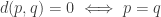
Proof. Let $p,q\in \mathbb{R}$ . Then by definition of $d(p,q)$ and by definition of the absolute value function, we have that $|p-q|\geq 0$ , so that axiom 1 is satisfied. Suppose now that the points in $\mathbb{R}$ are equal, i.e. that $p=q\in \mathbb{R}$ . Then by definition of 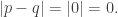$d(p,q)$ , we have that $|p-q|=|0|=0.$ Conversely, suppose that $|p-q|= 0.$ By the triangle inequality we have that 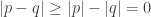$|p-q|\geq |p|-|q|=0$ This implies that $|p|= |q|$ . Thus, condition (2.) is satisfied and hence the distance between two points in $\mathbb{R}$ is zero if and only if the two points are the same. To prove condition (3.), let $p,q\in \mathbb{R}$ , so that $d(p,q) = |p-q|$ . By virtue of the definition of the absolute value, we can say that
$\displaystyle d(p,q) = |p-q| = |-(p+q)|= |-1||q-p|= |q-p|= d(q,p).$
Thus, we see that the arguments of the proposed distance function is symmetric with respect to its arguments, namely any real numbers $p,q\in \mathbb{R}$ . To prove condition (4.), consider any three points $p,q,r\in \mathbb{R}$ , then the distance function between the points $p,r \in \mathbb{R}$ becomes
$\displaystyle d(p,r) = |p-r| = |p-q+q-r|,$
wherein we add zero in the form of adding and subtracting the point q (a very common trick in analysis). Then by the properties of the absolute value it follows that
$\displaystyle d(p,r) = |p-q+q+r| \leq |p-q|+|q-r| = d(p,q)+d(q,r)$ ,
where by the last equality follows from the definition of the distance function. Therefore, all four conditions have been satisfied, and hence by our definition of a metric space, it follows that $(\mathbb{R},d)$ whose distance function $d:\mathbb{R}\times \mathbb{R}\rightarrow \mathbb{R}$ is defined by $d(p,q) = |p-q|$ is indeed a metric space. $\square$