The following post was initially one of my assignments for an independent study in modern physics in my penultimate year as an undergraduate. While studying this problem the text that I used to verify my answer was:
R. Eisberg and R. Resnick, Quantum Physics of Atoms, Molecules, Solids, Nuclei, and Particles. John Wiley & Sons. 1985. 6.
One of the hallmarks of quantum theory is the Schrödinger equation. There are two forms: the time-dependent and the time-independent equation. The former can be turned into the latter by way of assuming stationary states in which case there is no time evolution (i.e. the time derivative  .
.  denotes the derivative of the wavefunction
  with respect to time.)
The wavefunction describes the state of a system, and it is found by solving the Schrödinger equation. In this post, I’ll be considering a step potential in which
After solving for the wavefunction, I will calculate the reflection and transmission coefficients for the case where the energy of the electron is less than that of the step potential  .
.
First, we assume that we are dealing with stationary states, by doing so we assume that there is no time-dependence. The wavefunction becomes an eigenfunction (eigen– is German for “characteristic” e.g. characteristic function, characteristic value (eigenvalue), and so on),  . There are requirements for this eigenfunction in the context of quantum mechanics: eigenfunction and its first order spatial derivative
  must be finite, single-valued, and continuous. Using the wavefunction, we write the time-independent Schrödinger equation as

where  is the reduced Planck’s constant
  , m is the mass of the particle,
  represents the potential, and
  is the energy.
Now, in electron scattering there are two cases regarding a step potential: the case for which and the case for which  The focus of this post is the former case. In such a case, the potential is given mathematically by Eqs. (1.1) and (1.2) and can be depicted by the image below:
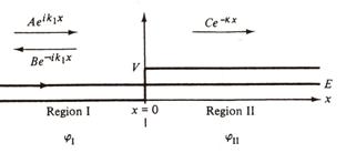
Image Credit: http://physics.gmu.edu/~dmaria/590%20Web%20Page/public_html/qm_topics/potential/barrier/STUDY-GUIDE.htm
The first part of this problem is to solve for when  . Then Eq.(2) becomes

where  . Eq.(3) is a second order linear homogeneous ordinary differential equation with constant coefficients and can be solved using a characteristic equation. We assume that the solution is of the general form

which upon taking the first and second order spatial derivatives and substituting into Eq.(3) yields

We can factor out the exponential and recalling that the graph of  (except in the limit
  )we can then conclude that
 .
.
Hence,  . Therefore, we can write the solution Schrödinger equation in the region
  as
as

This is the eigenfunction for the first region. Coefficients A and B will be determined later.
Now we can use the same logic for the Schrödinger equation in the region  where
where  :
:

where ![\kappa_{II}\equiv \frac{\sqrt[]{2m(E-V_{0})}}{\hbar}](https://s0.wp.com/latex.php?latex=%5Ckappa_%7BII%7D%5Cequiv+%5Cfrac%7B%5Csqrt%5B%5D%7B2m%28E-V_%7B0%7D%29%7D%7D%7B%5Chbar%7D&bg=ffffff&fg=333333&s=0&c=20201002) . The general solution for this region is
. The general solution for this region is

Now the next step is taken using two different approaches: the first using a mathematical argument and the other from a conceptual interpretation of the problem at hand. The former is this: Suppose we let  . What results is that the first term on the right hand side of Eq.(6) diverges (i.e. becomes arbitrarily large). The second term on the right hand side ends up going to zero (it converges). Therefore, D remains finite, hence
  . However, in order to suppress the divergence of the first term, we let
  . Thus we arrive at the eigenfunction for

The latter argument is this: In the region , the first term of the solution represents a wave propagating in the positive x-direction, while the second denotes a wave traveling in the negative x-direction. Similarly, in the region where , the first term corresponds to a wave traveling in the positive x-direction. However, this cannot be because the energy of the wave is not sufficient enough to overcome the potential. Therefore, the only term that is relevant here for this region is the second term, for it is a wave propagating in the negative x-direction.
We now determine the coefficients A and B. Recall that the eigenfunction must satisfy the following continuity requirements

evaluated when  . Doing so in Eqs. (4) and (7), and equating them we arrive at the continuity condition for
Taking the derivative of  and
and  and evaluating them for when we arrive at

If we add Eqs. (9) and (10) we get the value for the coefficient A in terms of the arbitrary constant D
Conversely, if we subtract (9) and (10) we get the value for B in terms of D

Now the reflection coefficient defined as

which is the probability that an incident electron (wave) will be reflected. On the other hand, the transmission coefficient is the probability that an electron will be transmitted through the potential (e.g. barrier potential). These two also must satisfy the relation
This means that the probability that the electron will be reflected or transmitted is 100%. Therefore, to evaluate R (the reason why I don’t calculate T will become apparent shortly), we take the complex conjugate of A and B and using them in Eq.(13) we get
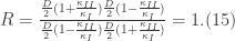
What this conceptually means is that the probability that the electron is reflected is 100%. This implies that it is impossible for an electron to be transmitted through the potential for this system.


 :
:
 so as not to confuse it with the notation for an ordinary derivative. Recall the Navier-Stokes’ equation and the vorticity equation

 and let
  and
and  . Then,


 multiplied by a volume element
  given by
 , the total derivative becomes an ordinary time derivative. Thus, Eq.(10) becomes
![\displaystyle \int_{V_{\omega}}\frac{d}{dt}(\textbf{u}\cdot \omega)dV=\iint_{S_{\omega}}\bigg\{\nabla \cdot [-\frac{P}{\rho}\omega + \frac{u^{2}}{2}\omega ]\bigg\}\cdot d\textbf{S}=0. (11)](https://s0.wp.com/latex.php?latex=%5Cdisplaystyle+%5Cint_%7BV_%7B%5Comega%7D%7D%5Cfrac%7Bd%7D%7Bdt%7D%28%5Ctextbf%7Bu%7D%5Ccdot+%5Comega%29dV%3D%5Ciint_%7BS_%7B%5Comega%7D%7D%5Cbigg%5C%7B%5Cnabla+%5Ccdot+%5B-%5Cfrac%7BP%7D%7B%5Crho%7D%5Comega+%2B+%5Cfrac%7Bu%5E%7B2%7D%7D%7B2%7D%5Comega+%5D%5Cbigg%5C%7D%5Ccdot+d%5Ctextbf%7BS%7D%3D0.+%2811%29&bg=ffffff&fg=333333&s=0&c=20201002)

 is the magnetic vector potential which is described by the following relations


 .
.
 represent the typical fluid velocity, length scale and typical volume respectively. The magnetic Reynolds number is the ratio between the advective and diffusive terms of the induction equation. There are two canoncial regimes: (1)
  , and (2)
 The former is sometimes called the diffusive limit and the latter is called either the Ideal limit or the infinite conductivity limit (I prefer to call it the ideal limit, since the terms infinite conductivity limit is not quite accurate).
 ) then we can use the aforementioned vector identity to write the induction equation as

 , in which case
 ) we may define the circulation as being
 , according to this theorem it states that this fluid element will continue to lie on that vortex line indefinitely.
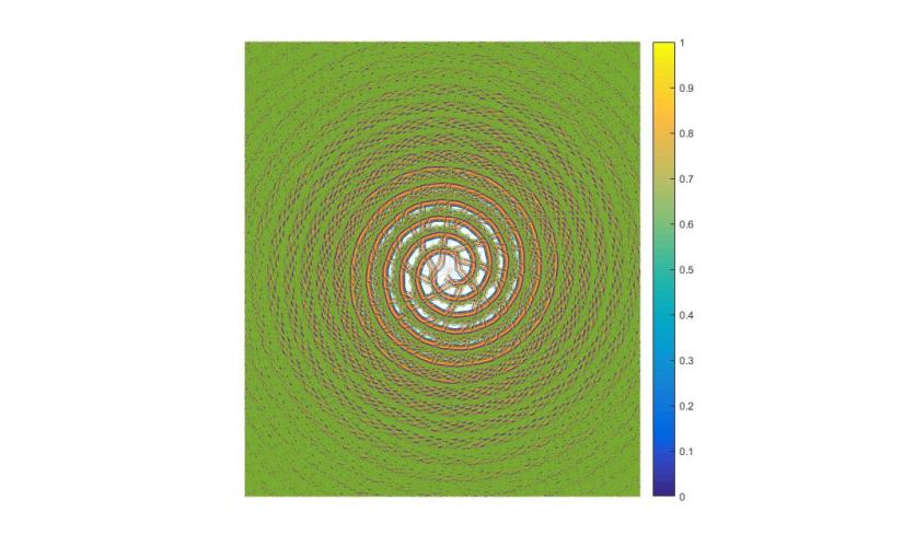
 passing through an area
  constrained to a solid angle
  in a time
  . We may write this mathematically as
 we get
 be an element of the surface
  in a volume
  through which radiation passes. Further let
  and
and  denote the angles which form normals with respect to elements
  . These surfaces are joined by these normals and hence we have the surface across which energy flows includes the elements
 is the solid angle subtended by the surface element
  and volume element
  is the volume that is intercepted in volume
 in the volume, then we must multiply Eq.(5) by
  , where
  is the speed of light.

 we get
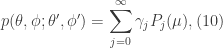
 represents the source function given by
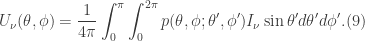
 (in keeping with our notation in

 . Furthermore, by the method of separation of variables we suppose that the solution is a product of eigenfunctions of the form
  . Hence, Laplace’s equation becomes
 into
into  . Rewriting (2) and multiplying by
 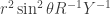 , we get
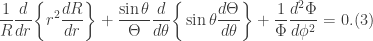
 , yielding
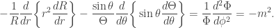

 and carry out the derivative in the angular component to get the Associated Legendre equation:
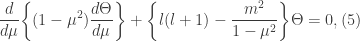
 . The solutions to this equation are known as the associated Legendre functions. However, instead of solving this difficult equation by brute force methods (i.e. power series method), we consider the case for which
  . In this case, Eq.(5) simplifies to Legendre’s differential equation discussed
 and for complex solutions
  , thus we can write the solutions as series whose indices run from 0 to l for the real-values and from -l to l for the complex-valued solutions.
 in place of the angular component, we get

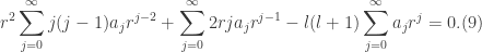
![\displaystyle \sum_{j=0}^{\infty}[j(j-1)+2j-l(l+1)]a_{j}r^{j}=0.](https://s0.wp.com/latex.php?latex=%5Cdisplaystyle+%5Csum_%7Bj%3D0%7D%5E%7B%5Cinfty%7D%5Bj%28j-1%29%2B2j-l%28l%2B1%29%5Da_%7Bj%7Dr%5E%7Bj%7D%3D0.&bg=ffffff&fg=333333&s=0&c=20201002)
 , this means that

 , we arrive at
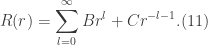
![\displaystyle \psi(r,\theta,\phi) = \sum_{l=0}^{\infty} \sum_{m=0}^{\infty}[Br^{l}+Cr^{-l-1}]\Theta_{l}^{m}(\mu)A\exp({im\phi}), (12)](https://s0.wp.com/latex.php?latex=%5Cdisplaystyle+%5Cpsi%28r%2C%5Ctheta%2C%5Cphi%29+%3D+%5Csum_%7Bl%3D0%7D%5E%7B%5Cinfty%7D+%5Csum_%7Bm%3D0%7D%5E%7B%5Cinfty%7D%5BBr%5E%7Bl%7D%2BCr%5E%7B-l-1%7D%5D%5CTheta_%7Bl%7D%5E%7Bm%7D%28%5Cmu%29A%5Cexp%28%7Bim%5Cphi%7D%29%2C%C2%A0+%2812%29&bg=ffffff&fg=333333&s=0&c=20201002)
![\displaystyle \psi(r,\theta,\phi)=\sum_{l=0}^{\infty}\sum_{m=-l}^{l}[Br^{l}+Cr^{-l-1}]\Theta_{l}^{m}(\mu)A\exp({im\phi}), (13)](https://s0.wp.com/latex.php?latex=%5Cdisplaystyle+%5Cpsi%28r%2C%5Ctheta%2C%5Cphi%29%3D%5Csum_%7Bl%3D0%7D%5E%7B%5Cinfty%7D%5Csum_%7Bm%3D-l%7D%5E%7Bl%7D%5BBr%5E%7Bl%7D%2BCr%5E%7B-l-1%7D%5D%5CTheta_%7Bl%7D%5E%7Bm%7D%28%5Cmu%29A%5Cexp%28%7Bim%5Cphi%7D%29%2C+%2813%29&bg=ffffff&fg=333333&s=0&c=20201002)


 ). It is nonphysical or nonsensical to speak of negative time.
 .At a time
  , the overall heat of the volume can be regarded to be a function
  . After a time period
  has passed, the heat will have traversed to the point
  Thus the initial-boundary-value-problem becomes
 . Also, this definition also reduces the three-dimensional laplacian to a second-order partial derivative of u. The boundary and initial conditions are then


 , so we can apply to the time dependence equation which then becomes

 allows us to write the spatial equation upon rearrangement as
![\alpha(\textbf{r})=c_{1}\cos({\sqrt[]{c\rho(\lambda^{2}+Q)}\textbf{r}})+c_{3}\sin({\sqrt[]{c\rho(\lambda^{2}+Q)}\textbf{r}}), (6.2)](https://s0.wp.com/latex.php?latex=%5Calpha%28%5Ctextbf%7Br%7D%29%3Dc_%7B1%7D%5Ccos%28%7B%5Csqrt%5B%5D%7Bc%5Crho%28%5Clambda%5E%7B2%7D%2BQ%29%7D%5Ctextbf%7Br%7D%7D%29%2Bc_%7B3%7D%5Csin%28%7B%5Csqrt%5B%5D%7Bc%5Crho%28%5Clambda%5E%7B2%7D%2BQ%29%7D%5Ctextbf%7Br%7D%7D%29%2C+%286.2%29&bg=ffffff&fg=333333&s=0&c=20201002)
 . Next we apply the boundary conditions. Let
  in
in  :
:![\alpha(0)=c_{1}+0=0 \implies c_{1}=0 \implies \alpha(\textbf{r})=C\sin(\sqrt[]{c\rho(\lambda^{2}+Q)} \textbf{r}). (7.1)](https://s0.wp.com/latex.php?latex=%5Calpha%280%29%3Dc_%7B1%7D%2B0%3D0+%5Cimplies+c_%7B1%7D%3D0+%5Cimplies+%5Calpha%28%5Ctextbf%7Br%7D%29%3DC%5Csin%28%5Csqrt%5B%5D%7Bc%5Crho%28%5Clambda%5E%7B2%7D%2BQ%29%7D+%5Ctextbf%7Br%7D%29.+%287.1%29&bg=ffffff&fg=333333&s=0&c=20201002)
 in (7.1) to get
![\alpha(R)\implies \sin({\sqrt[]{c\rho(\lambda^{2}+Q)}R})=0\implies \sqrt[]{c\rho(\lambda^{2}+Q)}R^{2}=(n\pi)^{2}.](https://s0.wp.com/latex.php?latex=%5Calpha%28R%29%5Cimplies+%5Csin%28%7B%5Csqrt%5B%5D%7Bc%5Crho%28%5Clambda%5E%7B2%7D%2BQ%29%7DR%7D%29%3D0%5Cimplies+%5Csqrt%5B%5D%7Bc%5Crho%28%5Clambda%5E%7B2%7D%2BQ%29%7DR%5E%7B2%7D%3D%28n%5Cpi%29%5E%7B2%7D.&bg=ffffff&fg=333333&s=0&c=20201002)
 above gives

 and using the solution for the time dependence, and also let the coefficients form a product equivalent to the indexed coefficient
  , we arrive at the solution for the heat equation:
 :
:

 represents a source of external forces,
  is the velocity field,
  is the pressure gradient,
  is the material density,
  is kinematic viscosity, and
  is the laplacian of the velocity field. More specifically, it is a consequence of the viscous stress tensor whose components can cause the parcel of fluid to experience stresses and strains.
 is the current density defined by Ohm’s law in a previous post, and also recall from
![\textbf{J}=\frac{1}{\mu_{0}\rho}[(\nabla \times \textbf{B})\times \textbf{B}], (4)](https://s0.wp.com/latex.php?latex=%5Ctextbf%7BJ%7D%3D%5Cfrac%7B1%7D%7B%5Cmu_%7B0%7D%5Crho%7D%5B%28%5Cnabla+%5Ctimes+%5Ctextbf%7BB%7D%29%5Ctimes+%5Ctextbf%7BB%7D%5D%2C+%284%29&bg=ffffff&fg=333333&s=0&c=20201002)
 is the permeability of free space. Now we invoke the vector identity
![[(\nabla \times \textbf{B})\times \textbf{B}]=(\nabla \cdot \textbf{B})\textbf{B}-\nabla \bigg\{\frac{B^{2}}{2}\bigg\}. (5)](https://s0.wp.com/latex.php?latex=%5B%28%5Cnabla+%5Ctimes+%5Ctextbf%7BB%7D%29%5Ctimes+%5Ctextbf%7BB%7D%5D%3D%28%5Cnabla+%5Ccdot+%5Ctextbf%7BB%7D%29%5Ctextbf%7BB%7D-%5Cnabla+%5Cbigg%5C%7B%5Cfrac%7BB%5E%7B2%7D%7D%7B2%7D%5Cbigg%5C%7D.+%285%29&bg=ffffff&fg=333333&s=0&c=20201002)
 The Navier-Stokes’ equation becomes the Euler equation at this point. (Despite great understanding of classical mechanics, one phenomena for which we cannot account is turbulence and sources of friction, so this assumption is made out of necessity as well as simplicity. For processes in which turbulence cannot be neglected the best we can do in this regard is to parameterize turbulence in numerical models.) Using the vector identity as well as making use of our assumption of laminar flows, ideal one-fluid momentum equation is
 is the magnetic pressure exerted on magnetic field lines and the additional term
  is the magnetic tension acting along the magnetic field lines.