Consequences and some Elementary Theorems of the Ideal One-Fluid Magnetohydrodynamic Equations

SOURCE FOR CONTENT:

Priest, E. Magnetohydrodynamics of the Sun, 2014. Cambridge University Press. Ch.2.;

Davidson, P.A., 2001. An Introduction to Magnetohydrodynamics. Ch.4.

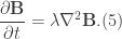
We have seen how to derive the induction equation from Maxwell’s equations assuming no charge and assuming that the plasma velocity is non-relativistic. Thus, we have the induction equation as being

$\displaystyle \frac{\partial \textbf{B}}{\partial t}=\nabla \times (\textbf{v}\times \textbf{B})+\lambda \nabla^{2}\textbf{B}. (1)$

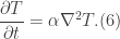
Many texts in MHD make the comparison of the induction equation to the vorticity equation

$\displaystyle \frac{\partial \Omega}{\partial t}= \nabla \times (\textbf{v} \times \Omega)+\nu \nabla^{2}\Omega, (2)$

where I have made use of the vector identity

$\nabla \times (\textbf{X}\times \textbf{Y})=\textbf{X}(\nabla \cdot \textbf{Y})-\textbf{Y}(\nabla \cdot \textbf{X})+(\textbf{Y}\cdot \nabla)\textbf{X}-(\textbf{X}\cdot \nabla)\textbf{Y}$ .

Indeed, if we do compare the induction equation (Eq.(1)) to the vorticity equation (Eq.(2)) we easily see the resemblance between the two. The first term on the right hand side of Eq.(1)/ Eq.(2) determines the advection of magnetic field lines/vortex field lines; the second term on the right hand side deals with the diffusion of the magnetic field lines/vortex field lines.

From this, we can impose restrictions and thus look at the consequences of the induction equation (since it governs the evolution of the magnetic field). Furthermore, we see that we can modify the kinematic theorems of classical vortex dynamics to describe the properties of magnetic field lines. After discussing the direct consequences of the induction equation, I will discuss a few theorems of vortex dynamics and then introduce their MHD analogue.

Inherent to this is magnetic Reynold’s number. In geophysical fluid dynamics, the Reynolds number (not the magnetic Reynolds number) is a ratio between the viscous forces per volume and the inertial forces per volume given by

$\displaystyle Re=\frac{ul}{V}, (3)$

where $u, l, V$ represent the typical fluid velocity, length scale and typical volume respectively. The magnetic Reynolds number is the ratio between the advective and diffusive terms of the induction equation. There are two canoncial regimes: (1) $Re_{m}<<1$ , and (2) $Re_{m}>>1$ The former is sometimes called the diffusive limit and the latter is called either the Ideal limit or the infinite conductivity limit (I prefer to call it the ideal limit, since the terms infinite conductivity limit is not quite accurate).

Case I: $Re_{m}<<1$

Consider again the induction equation

$\displaystyle \frac{\partial \textbf{B}}{\partial t}=\nabla \times (\textbf{v}\times \textbf{B})+\lambda\nabla^{2}\textbf{B}.$

If we then assume that we are dealing with incompressible flows (i.e. $(\nabla \cdot \textbf{v})=0$ ) then we can use the aforementioned vector identity to write the induction equation as

$\displaystyle \frac{D\textbf{B}}{Dt}=(\textbf{B}\cdot \nabla)\textbf{v}+\lambda\nabla^{2}\textbf{B}. (4)$

In the regime for which $Re_{m}<<1$ , the induction equation for incompressible flows (Eq.(4)) assumes the form

$\displaystyle \frac{\partial \textbf{B}}{\partial t}=\lambda \nabla^{2}\textbf{B}. (5)$

Compare this now to the following equation,

$\displaystyle \frac{\partial T}{\partial t}=\alpha \nabla^{2}T. (6)$

We see that the magnetic field lines are diffused through the plasma.

Case II: $Re_{m}>>1$

If we now consider the case for which the advective term dominates, we see that the induction equation takes the form

$\displaystyle \frac{\partial \textbf{B}}{\partial t}=\nabla \times (\textbf{v}\times \textbf{B}). (7)$

Mathematically, what this suggests is that the magnetic field lines become “frozen-in” the plasma, giving rise to Alfven’s theorem of flux freezing.

Many astrophysical systems require a high magnetic Reynolds number. Such systems include the solar magnetic field (heliospheric current sheet), planetary dynamos (Earth, Jupiter, and Saturn), and galactic magnetic fields.

Kelvin’s Theorem & Helmholtz’s Theorem:

Kelvin’s Theorem: Consider a vortex tube in which we have that $(\nabla \cdot \Omega)=0$ , in which case

$\displaystyle \oint \Omega \cdot d\textbf{S}=0, (8)$

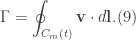
and consider also the curve taken around a closed surface, (we call this curve a material curve $C_{m}(t)$ ) we may define the circulation as being

$\displaystyle \Gamma = \oint_{C_{m}(t)}\textbf{v}\cdot d\textbf{l}. (9)$

Thus, Kelvin’s theorem states that if the material curve is closed and it consists of identical fluid particles then the circulation, given by Eq.(9), is temporally invariant.

Helmholtz’s Theorem:

Part I: Suppose we consider a fluid element which lies on a vortex line at some initial time $t=t_{0}$ , according to this theorem it states that this fluid element will continue to lie on that vortex line indefinitely.

Part II: This part says that the flux of vorticity

$\displaystyle \Phi = \int \Omega \cdot d\textbf{S}, (10)$

remains constant for each cross-sectional area and is also invariant with respect to time.

Now the magnetic analogue of Helmholtz’s Theorems are found to be Alfven’s theorem of flux freezing and conservation of magnetic flux, magnetic field lines, and magnetic topology.

The first says that fluid elements which lie along magnetic field lines will continue to do so indefinitely; basically the same for the first Helmholtz theorem.

The second requires a more detailed argument to demonstrate why it works but it says that the magnetic flux through the plasma remains constant. The third says that magnetic field lines, hence the magnetic structure may be stretched and deformed in many ways, but the magnetic topology overall remains the same.

The justification for these last two require some proof-like arguments and I will leave that to another post.

In my project, I considered the case of high magnetic Reynolds number in order to examine the MHD processes present in region of metallic hydrogen present in Jupiter’s interior.

In the next post, I will “prove” the theorems I mention and discuss the project.

Share this:

Like this:

Related

Leave a Reply Cancel reply