Solution to the three-dimensional Heat Equation

After taking a topics course in applied mathematics (partial differential equations), I found that there were equations that I should solve since I would later see those equations embedded into other larger-scale equations. This equation was Laplace’s equation (future post). Once I solved this equation, I realized that it becomes a differential operator when acted upon a function of at least two variables. Thus, I could solve equations such as the Schrödinger equation using a three-dimensional laplacian in spherical-polar coordinates (another future post) and the three-dimensional heat equation. I will be solving the latter.

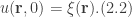
The heat equation initial-boundary-value-problem is therefore

$\frac{\partial u}{\partial t}=\frac{1}{c\rho}\nabla^{2}u+Q(x,y,z), (1.1)$

subjected to the boundary conditions

$u(0,0,0,t)=0, (1.2)$

and the initial condition

$u(x,y,z,0)= \xi(x,y,z). (1.8)$

Now, this solution is not specific to a single thermodynamic system, but rather it is a more general solution in a mathematical context. However, I will be appropriating certain concepts from physics for reasons that are well understood (i.e. that time exists on the interval $I=0\leq t < +\infty$ ). It is nonphysical or nonsensical to speak of negative time.

To start, consider any rectangular prism in which heat flows through the volume, from the origin to the point $(X,Y,Z)$ .At a time $t=0$ , the overall heat of the volume can be regarded to be a function $\xi(x,y,z)$ . After a time period $\delta t=t$ has passed, the heat will have traversed to the point $(X,Y,Z)$ from the origin (think of the heat traveling along the diagonal of a cube). The goal is to find the heat as a function of the three spatial components and a single time component. Furthermore, the boundary conditions maintain that at the origin and the final point, the heat vanishes. In other words, these points act as heat sinks. (A sink is a point where energy can leave the system.)

To simplify the notation, we define $\textbf{r}=x\hat{i}+y\hat{j}+z\hat{k}.$ Thus the initial-boundary-value-problem becomes

$\frac{\partial u}{\partial t}=\frac{1}{c\rho}\frac{\partial^{2}u}{\partial \textbf{r}^{2}}, (2.1)$

where $u\rightarrow u(\textbf{r},t)$ . Also, this definition also reduces the three-dimensional laplacian to a second-order partial derivative of u. The boundary and initial conditions are then

$u(0,t)=0,(2.2)$

$u(R,t)=0, (2.3)$

$u(\textbf{r},0)=\xi(\textbf{r}). (2.2)$

Now, we assume that the solution is a product of eigenfunctions of the form

$u(\textbf{r},t)=\alpha(\textbf{r})\Gamma(t). (3)$

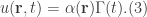
Taking the respective derivatives and dividing by the assumed form of the solution, we get

$\frac{\Gamma^{\prime}(t)}{\Gamma(t)}=\frac{1}{c\rho}\frac{\alpha^{\prime\prime}(\textbf{r})}{\alpha(\textbf{r})}+Q(\textbf{r}). (4)$

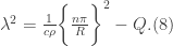
Now, Eq.(4) can be equal to three different values, the first of which is zero, but this solution does not help in any way, nor is it physically significant since it produces a trivial solution. The second is $\lambda^{2}>0, \lambda \neq 0$ , so we can apply to the time dependence equation which then becomes

$\frac{\Gamma^{\prime}(t)}{\Gamma(t)}=\lambda^{2}, (5.1)$

whose solution is

$\Gamma(t)=\Gamma_{0}\exp({\lambda^{2}t}). (5.2)$

The third case where $\lambda^{2}<0, \lambda \neq 0$ allows us to write the spatial equation upon rearrangement as

$\alpha^{\prime\prime}(\textbf{r})+c\rho(\lambda^{2}+Q)\alpha(\textbf{r})=0, (6.1)$

whose solution is

$\alpha(\textbf{r})=c_{1}\cos({\sqrt[]{c\rho(\lambda^{2}+Q)}\textbf{r}})+c_{3}\sin({\sqrt[]{c\rho(\lambda^{2}+Q)}\textbf{r}}), (6.2)$

where $c_{3}=-c_{2}$ . Next we apply the boundary conditions. Let $\textbf{r}=0$ in $\alpha(\textbf{r})$ :

$\alpha(0)=c_{1}+0=0 \implies c_{1}=0 \implies \alpha(\textbf{r})=C\sin(\sqrt[]{c\rho(\lambda^{2}+Q)} \textbf{r}). (7.1)$

and let $\textbf{r}=R$ in (7.1) to get

$\alpha(R)\implies \sin({\sqrt[]{c\rho(\lambda^{2}+Q)}R})=0\implies \sqrt[]{c\rho(\lambda^{2}+Q)}R^{2}=(n\pi)^{2}.$

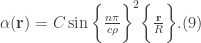
Solving for $\lambda^{2}$ above gives

$\lambda^{2}=\frac{1}{c\rho}\bigg\{\frac{n\pi}{R}\bigg\}^{2}-Q. (8)$

Substituting into Eq.(7.1) and simplifying gives

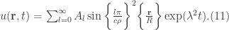
$\alpha(\textbf{r})=C\sin\bigg\{\frac{n\pi}{c\rho}\bigg\}^{2}\bigg\{\frac{\textbf{r}}{R}\bigg\}. (9)$

To find as many solutions as possible we construct a superposition of solutions of the form

$u(\textbf{r},t)=u_{l}(\textbf{r},t)=\sum_{l=0}^{\infty}\alpha_{l}(\textbf{r})\Gamma(t). (10)$

Rewriting $\alpha(\textbf{r})$ as $\alpha_{l}(\textbf{r})$ and using the solution for the time dependence, and also let the coefficients form a product equivalent to the indexed coefficient $A_{l}$ , we arrive at the solution for the heat equation:

$u(\textbf{r},t)=\sum_{l=0}^{\infty}A_{l}\sin\bigg\{\frac{l\pi}{c\rho}\bigg\}^{2}\bigg\{\frac{\textbf{r}}{R}\bigg\}\exp(\lambda^{2}t). (11)$

Now suppose that $t=0$ in Eq.(11). In this case we get the initial heat distribution given by $\xi(\textbf{r})$ :

$\xi(\textbf{r})=\sum_{l=0}^{\infty} A_{l}\sin\bigg\{\frac{l\pi}{c\rho}\bigg\}^{2}\bigg\{\frac{\textbf{r}}{R}\bigg\}. (12)$

Share this:

Like this:

Related

Leave a Reply Cancel reply