Simple Harmonic Oscillators (SHOs) (Part I)

We all experience or see this happening in our everyday experience: objects moving back and forth. In physics, these objects are called simple harmonic oscillators. While I was taking my undergraduate physics course, one of my favorite topics was SHOs because of the way the mathematics and physics work in tandem to explain something we see everyday. The purpose of this post is to engage followers to get them to think about this phenomenon in a more critical manner.

Every object has a position at which these objects tend to remain at rest, and if they are subjected to some perturbation, that object will oscillate about this equilibrium point until they resume their state of rest. If we pull or push an object with an applied force $F_{A}$ we find that this force is proportional to Hooke’s law of elasticity, that is, $F_{A}=-k\textbf{r}$ . If we consider other forces we also find that there exists a force balance between the restoring force (our applied force), a resistance force, and a forcing function, which we assume to have the form

$F=F_{forcing}+F_{A}-F_{R}= -k\textbf{r}-\beta \dot{\textbf{r}}; (1)$

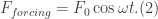
note that we are assuming that the resistance force is proportional to the speed of an object. Suppose further that we are inducing these oscillations in a periodic manner by given by

$F_{forcing}=F_{0}\cos{\omega t}. (2)$

Now, to be more precise, we really should define the position vector. So, $\textbf{r}=x\hat{i}+y\hat{j}+z\hat{k}$ . Therefore, we actually have a system of three second order linear non-homogeneous ordinary differential equations in three variables:

$m\ddot{ x}+\beta \dot{x}+kx=F_{0}\cos{\omega t}, (3.1)$

$m\ddot{y}+\beta \dot{y}+ky=F_{0}\cos{\omega t}, (3.2)$

$m\ddot{z}+\beta \dot{z}+kz=F_{0}\cos{\omega t}. (3.3)$

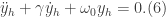
(QUICK NOTE: In the above equations, I am using the Newtonian notation for derivatives, only for convenience.) I will just make some simplifications. I will divide both sides by the mass, and I will define the following parameters: $\gamma \equiv \beta/m$ , $\omega_{0} \equiv k/m$ , and $\alpha \equiv F_{0}/m$ . Furthermore, I am only going to consider the $y$ component of this system. Thus, the equation that we seek to solve is

$\ddot{y}+\gamma \dot{y}+\omega_{0}y=\alpha\cos{\omega t}. (4)$

Now, in order to solve this non-homogeneous equation, we use the method of undetermined coefficients. By this we mean to say that the general solution to the non-homogeneous equation is of the form

$y = Ay_{1}(t)+By_{2}(t)+Y(t), (5)$

where $Y(t)$ is the particular solution to the non-homogeneous equation and the other two terms are the fundamental solutions of the homogeneous equation:

$\ddot{y}_{h}+\gamma \dot{y}_{h}+\omega_{0} y_{h} = 0. (6)$

Let $y_{h}(t)=D\exp{(\lambda t)}$ . Taking the first and second time derivatives, we get $\dot{y}_{h}(t)=\lambda D\exp{(\lambda t)}$ and $\ddot{y}_{h}(t)=\lambda^{2}D\exp{(\lambda t)}$ . Therefore, Eq. (6) becomes, after factoring out the exponential term,

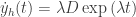
$D\exp{(\lambda t)}[\lambda^{2}+\gamma \lambda +\omega_{0}]=0. (7)$

Since $D\exp{(\lambda t)}\neq 0$ , it follows that

$\lambda^{2}+\gamma \lambda +\omega_{0}=0. (8)$

This is just a disguised form of a quadratic equation whose solution is obtained by the quadratic formula:

$\lambda =\frac{-\gamma \pm \sqrt[]{\gamma^{2}-4\omega_{0}}}{2}. (9)$

Part II of this post will discuss the three distinct cases for which the discriminant $\sqrt[]{\gamma^{2}-4\omega_{0}}$ is greater than, equal to , or less than 0, and the consequent solutions. I will also obtain the solution to the non-homogeneous equation in that post as well.

Share this:

Like this:

Related

Leave a Reply Cancel reply