While I was in school, one of my professors set this problem to me and my classmates and challenged us to solve it over the next few days. I found the challenge intriguing and it fascinated me, so I thought it was worth sharing. The problem was this:
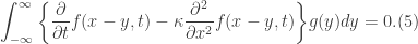
Show that
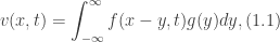
where 

First off, what does finite support mean? Mathematically speaking, a function has support which is characterized by a subset of its domain whose members do not map to zero, and yet are finite. (Just as a quick note: much of the proper definitions require an understanding in mathematical analysis and measure theory, something which I have not studied in detail, so take that explanation with a grain of salt.)
As for the solution, we can rewrite the given PDE as
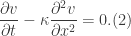
The PDE requires a first-order time derivative and a second-order spatial derivative.
and

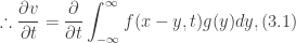
Next, we substitute Eqs. (3.1) and (3.2) into Eq.(2), yielding

Note that taking the derivative of a function and then integrating that function is equivalent to integrating the function and differentiating the same function, in conjunction with the fact that the sum or difference of the integrals is the integral of the sum or difference (proofs of these facts are typically covered in a course in real analysis). Taking advantage of these gives
Notice that the terms contained in the brackets equate to 
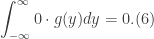
This implies that the function 
References:
Definition of Support in Mathematics: https://en.wikipedia.org/wiki/Support_(mathematics)

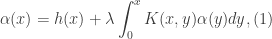
![y\in [0,x]](https://s0.wp.com/latex.php?latex=y%5Cin+%5B0%2Cx%5D&bg=ffffff&fg=333333&s=0&c=20201002) . The first term of the integrand
. The first term of the integrand  denotes the kernel. The kernel of the integral arises from its conversion from an initial value problem. Indeed, solving the integral equation is equivalent to solving the initial value problem of a differential equation. The integral equation includes the initial conditions instead of being added in near the end of the solution of an IVP.
 Then the next iteration of
  is
is
 is
is


 is determined, we may determine the exact solution
  via
via
