Physics – Understanding Physics and Astronomy

A PROBLEM IN THERMODYNAMICS AND STATISTICAL MECHANICS: ANALYTICAL AND NUMERICAL STUDY OF AN EINSTEIN SOLID-Analytical Solution

IMAGE CREDIT/OBTAINED FROM: https://mappingignorance.org/2015/12/17/einstein-and-quantum-solids/

Quite some time ago, I had posted a numerical study of an Einstein solid and I now present the analytical study of an Einstein solid. As this was one problem in one of my problem sets while studying thermodynamics and statistical mechanics, one may find this exact problem in the following text:

Schroeder D.V., An Introduction to Thermal Physics, (2000). Addison Wesley Longman. Chapter 3: Interactions and Implications: Problem 3.25. pp. 108.

What I will be presenting is my solution to this problem and I will be offering my interpretation of the problem statement and the implications of the solution.

We begin with the provided approximation,

$\displaystyle \Omega(N,q)\approx \bigg(\frac{q+N}{q}\bigg)^{q}\bigg(\frac{q+N}{N}\bigg)^{N}. (1)$

This expression represents the multiplicity of an Einstein solid with $N$ oscillators and $q$ energy units. Recall that the equation to find the entropy is the following

$\displaystyle S=k\ln{(\Omega(N,q))}. (2)$

Thus, upon substitution of the multiplicity (Eq.(1)) into the equation for entropy (Eq.(2)), one arrives at the equation

$\displaystyle S=k\ln{\bigg\{\bigg(\frac{q+N}{q}\bigg)^{q}\bigg(\frac{q+N}{N}\bigg)^{N}\bigg\}}. (3)$

Upon making use of the properties of logarithms, we may write the equation equivalently as

$\displaystyle S = k\ln{\bigg\{\bigg(\frac{q+N}{q}\bigg)^{q}\bigg\}}+k\ln{\bigg\{(\frac{q+N}{N}\bigg)^{N}\bigg\}}, (4)$

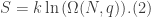
and again using the well-known property that $\ln{x}^{a}=a\ln{x}$ , we may further simplify Eq.(4) such that we arrive at the expression for the entropy of an Einstein solid:

$\displaystyle S = kq\ln{\bigg\{\bigg(\frac{q+N}{q}\bigg)\bigg\}}+Nk\ln{\bigg\{\bigg(\frac{q+N}{N}\bigg)\bigg\}}. (5)$

We may omit the factor of $(2\pi q(q+N))^{1/2}N^{-1/2}$ from Stirling’s approximation owing to the fact that if $N$ and $q$ are very large numbers, then $\sqrt{q}<<q$ and $\sqrt{N}<<N$ . Hence, it follows that $\sqrt{q+N}<<(q+N)$ . So we see that the aforementioned factor is of no consequence provided that $q$ and $N$ (i.e. the number of energy units and oscillators) is very large.

The second part of this problem asks to take the expression we derived for the entropy and compute the temperature. Recall that the definition for temperature is given by the equation

$\displaystyle \frac{1}{T}=\bigg(\frac{\partial S}{\partial U}\bigg)^{-1}. (6)$

From substitution we may write the following

$\displaystyle \frac{1}{T}=\bigg\{\frac{\partial}{\partial U}\bigg(k\bigg(\frac{U}{\epsilon}+N\bigg)\ln{\bigg(\frac{U}{\epsilon}+N\bigg)}\bigg)-\frac{\partial}{\partial U}\bigg(\frac{kU}{\epsilon}\ln{\bigg(\frac{U}{\epsilon}\bigg)}\bigg)-\frac{\partial}{\partial U} (N\ln{(N))}\bigg\}^{-1}, (7)$

where I have made use of the properties of logarithms and made the substitution $q=U/\epsilon$ . Differentiating and simplifying yields,

$\displaystyle \frac{1}{T}=\bigg\{\bigg(\frac{k}{\epsilon}\bigg)\ln{\bigg(\frac{U}{\epsilon}+N\bigg)}-\ln{\bigg(\frac{U}{\epsilon}\bigg)}\bigg\}^{-1}. (8)$

Further simplification yields the equation for temperature $T$ of an Einstein solid

$\displaystyle T = \frac{\epsilon}{k\ln{\bigg(\frac{U+\epsilon N}{U}}\bigg)}. (9)$

Part three asks us to find the equation for the heat capacity from our temperature equation. Recall that the equation for heat capacity is of the form

$\displaystyle C = \bigg(\frac{\partial U}{\partial T}\bigg). (10)$

However, we need an equation for the internal energy $U$ as a function of temperature $T$ . We actually have the opposite. So we must solve Eq.(9) for the internal energy, and doing so yields

$\displaystyle U(T)=\frac{\epsilon N}{\exp{(\epsilon/kT)}-1}. (11)$

Substituting Eq.(11) into Eq.(10) gives

$\displaystyle C = \bigg(\frac{\partial U}{\partial T}\bigg)=\frac{\partial}{\partial T}\bigg(\frac{\epsilon N}{\exp{(\epsilon/kT)}-1}\bigg). (12)$

Using the quotient rule for derivatives gives the equation for the heat capacity

$\displaystyle C =\bigg(\frac{\epsilon^{2}N}{kT^{2}}\bigg) \bigg(\frac{\exp{(\epsilon/kT)}}{{(\exp{(\epsilon/kT)}-1)}^{2}}\bigg). (13)$

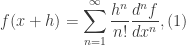
The next part asked to show that in the limit $T \rightarrow \infty$ , the heat capacity $C =Nk$ . Recall that the Taylor series expansion for the exponential function $\exp{(x)}$ is given by

$\displaystyle \exp{(x)}=\sum_{j=0}^{\infty}\frac{x^{j}}{j!}. (14)$

For small values of $x$ we may make the approximation $\exp{(x)}\approx 1+ x$ . Then we have the approximate relation

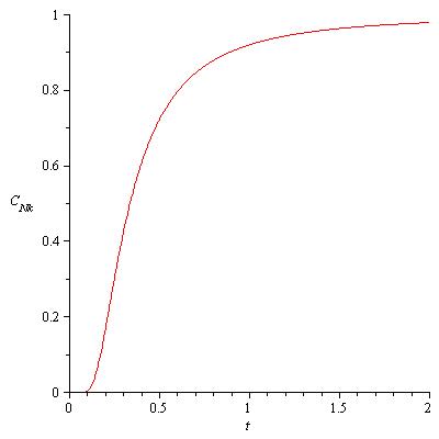
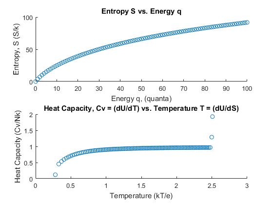
$\displaystyle C \approx \frac{\epsilon^{2}N}{kT^{2}}\frac{(1+\epsilon/kT)}{(1+(\epsilon/kT)-1)^{2}}=\frac{\epsilon^{2}N(1+(\epsilon/kT))}{kT^{2}(\epsilon^{2}/k^2 T^2)}= Nk(1+(\epsilon/kT)). (15)$

Then considering the aforementioned limit yields

$\displaystyle \lim_{T \rightarrow \infty} C = \lim_{T \rightarrow \infty} \bigg(Nk(1+(\epsilon/kT))\bigg)= Nk. (16)$

The final part of my solution to this problem (I did not complete the last portion of the problem see the aforementioned reference for the problem) asks us to graph the resultant equation relating the heat capacity and the temperature. Below is a plot of the function in the technical computing software Maple.

Fig.1 Heat Capacity vs. Temperature

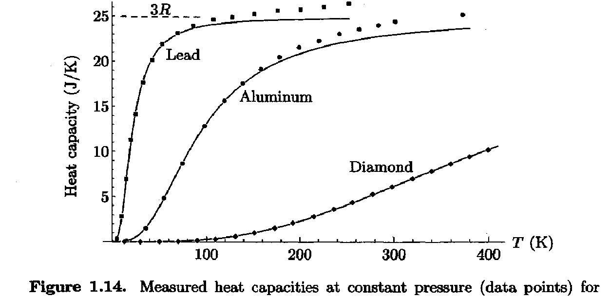
For low temperatures, the heat capacity initially starts at $0$ . However, when $t=0.097$ , there appears to be a dramatic increase in the heat capacity in the dimensionless quantity $C/Nk$ . If the heat capacity $C$ is graphed as a function of temperature $T$ , and one uses the $\epsilon$ values for each of the lead and aluminum curves produced in Fig. 1.14 of Schroeder’s An Introduction to Thermal Physics.

Let me know if I made any mistakes anywhere, and I will do my best to correct them.

Clear skies!

Basics of Tensor Calculus & General Relativity|A Digression into Special Relativity

So far in this series I have given the definitions of vectors, scalars, tensors, and manifolds. As a result, much of this series has been mostly mathematics and not necessarily physics. To that end, the purpose of this post is to develop the salient points of special relativity. Namely, the intention of this post is to cover the following:

Definition of Inertial Reference Frames: Standard Configuration and Einstein’s Postulates.
Development of the Lorentz Transformation Matrix
Discussion of the Newtonian geometry of spacetime
Discussion of the Minkowski geometry of spacetime (i.e. no curvature)
Finally I will show that the quantity $\delta s^{2}$ is invariant with respect to Lorentz transformations. This is a pretty standard problem in most GR textbooks and in fact in some introductory books on SR.

Continue reading Basics of Tensor Calculus & General Relativity|A Digression into Special Relativity

Basics of Tensor Calculus and General Relativity: An Introduction to Manifolds and Coordinates

SOURCE FOR CONTENT: General Relativity: An Introduction for Physicists, Hobson, M.P., Efsttathiou, G., and Lasenby, A.N., 2006. Cambridge University Press.

D-Dimensional Hypersphere and Gamma Function: Introduction to Thermal Physics, Schroeder D.V. 2000. Addison-Wesley-Longmann.

IMAGE CREDIT: NASA/JPL.

The intended purpose of the post is to introduce the concept of manifolds in the context of physics (mathematicians beware!). Furthermore, I will discuss the concepts of Riemannian and pseudo-Riemannian manifolds before moving on towards tensors. This will be the first post in this topic of the series. In order to properly discuss the concepts of general relativity, I will have to break up this part of the series into smaller posts.

Part I. In this part of the series, I will discuss the concept of a tensor, and then discuss the introductory topics of manifolds.

A topic that has long eluded a conceptual understanding on my part is a tensor. In the first post of the series we saw a very technical and quite frustrating definition of a tensor. I have read numerous treatments and watched a number of lectures and videos and based on everything I have encountered, here is my understanding of a tensor as of writing this post…

Tensors are geometric objects that can be viewed in a similar way as one views matrices, whose elements are components of the tensor, and will have an overall value. More specifically, a tensor will take two geometric objects as inputs and will give you a scalar (a real number). Furthermore, under a transformation or in a different reference frame, the scalar that the tensor outputs will remain the same in all frames. The objects that change are, in fact, the components of the tensor. These components must obey specific transformation equations so as to preserve the scalar quantity of produced by the tensor. In more mathematical sense, a tensor is a mapping of a number of vectors (including 1-forms and the like) into the real number ordered field.

(**This is the best definition that I could come up with in order to define in a more satisfactory way a tensor.**)

Manifolds

According to the aforementioned reference, a manifold in its most general sense, is any set that one can describe by specifying parameters continuously. In the context of physics, we deal with differentiable manifolds.

A differentiable manifold is a continuous collection of points where each point is differentiable. This definition isn’t any better than the initial definition of a tensor. So, to elaborate a bit, we shall define the concept of continuity: a manifold is continuous if in the local region of a point $n_{1}$ , there exists points whose difference relative to $n_{1}$ is $dn$ .

From this, we can say that a differentiable manifold is a manifold for which we can ascribe to it a scalar field containing points at which it is possible to take derivatives of all orders.

Some examples include: 3-Dimensional Euclidean Space and Phase Space.

3-Dimensional Space

This differentiable manifold requires 3 coordinates (parameters) to specify a single point in the space. Since it requires three parameters the dimension of this particular manifold is 3. Mathematicians sometimes call this 3-space.

Phase Space

This is a manifold that one encounters more often in physics. I came across this manifold (although I did not refer to it as such) while taking my thermodynamics and statistical mechanics course. I found that this manifold requires 6 parameters in order to specify any point. Typically, these parameters include positions (or one radius vector) and velocities or momenta.

A submanifold or surface that I found applicable to phase space would be the $D$ -dimensional hypersphere whose surface area is given by

$\displaystyle A_{d}(r)=\frac{2\pi^{d/2}}{(\frac{d}{2}-1)!}r^{d-1}=\frac{2\pi^{d/2}}{\Gamma(\frac{d}{2})}r^{d-1}, (1)$

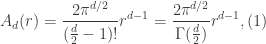
where $\Gamma(\frac{d}{2})$ is the gamma function given by

$\displaystyle \Gamma(d+1)\equiv \int_{0}^{\infty}x^{d}\exp{(-x)}dx. (2)$

To be more precise, the surface area (Eq.1) of this hypersphere is technically the volume of momentum space, but I am including to present a more concrete example of a manifold.

The next post will make the concepts mentioned here a bit more quantitative. This post was really just to introduce a more conceptual understanding.

Clear skies!

Astrophysics Series: Derivation of the Total Energy of a Binary Orbit

SOURCE FOR CONTENT: An Introduction to Modern Astrophysics, Carroll & Ostlie, Cambridge University Press. Ch.2 Celestial Mechanics

Here is my solution to one of the problems in the aforementioned text. I derive the total energy of a binary system making use of center-of-mass coordinates. In order to conceptualize it I have used the binary Alpha Centauri A and Alpha Centauri B. While writing this I stumbled upon the Kepler problem, the two-body problem, and the N-body problem. Leave a comment if you would like me to consider that in another post.

Clear Skies!

Derivation of the Total Energy of a Binary Orbit:

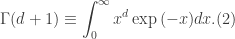
Setup: Consider the nearest binary star system to our solar system: Alpha Centauri A and Alpha Centauri B. These two stars orbit each other about a common center of mass; a point called a barycenter. The orbital radius vector of Alpha Centauri A is $\textbf{r}_{1}$ and the orbital radius vector of Alpha Centauri B is $\textbf{r}_{2}$ . The masses of Alpha Centauri A and B are $m_{1}$ , and $m_{2}$ , respectively. The total mass of the binary orbit $M$ is the sum of the individual masses of each component. In the context of this system, we encounter what is called the two-body problem of which there exists a special case known as the Kepler Problem (by the way let me know if that would be something that you guys would want to see…). We can simplify this two-body problem by making use of center-of-mass coordinates wherein we define the reduced mass $\mu$ . Therefore, the derivation of the total energy of the binary system of Alpha Centauri A and B will be carried out in such a coordinate system.

To derive this energy equation, one would typically make use of center-of-mass coordinates in which

$\displaystyle \textbf{r}_{1}=-\frac{\mu}{m_{1}}r, (0.1)$

and

$\displaystyle \textbf{r}_{2}=\frac{\mu}{m_{2}}r, (0.2)$

where $\mu$ represents the reduced mass given by

$\displaystyle \mu\equiv \frac{m_{1}m_{2}}{m_{1}+m_{2}}=\frac{m_{1}m_{2}}{M}. (0.3)$

Recall from conservation of energy that

$\displaystyle E = \frac{1}{2}m_{1}\dot{r}_{1}^{2}+\frac{1}{2}m_{2}\dot{r}_{2}^{2}-G\frac{m_{1}m_{2}}{|\mathcal{R}|}, (1)$

where $|\mathcal{R}|$ represents the separation distance between the two components. Let us take the derivative of Eqs.(0.1) and (0.2) to get

$\displaystyle \dot{r}_{1}=-\frac{\mu}{m_{1}}v, (2.1)$

and

$\displaystyle \dot{r}_{2}= \frac{\mu}{m_{2}}v. (2.2)$

Substitution yields

$\displaystyle E = \frac{1}{2}\frac{\mu^{2}}{m_{1}}v^{2}+\frac{1}{2}\frac{\mu^{2}}{m_{2}}v^{2}-G\frac{m_{1}m_{2}}{|\mathcal{R}|}. (3)$

Upon making use of the definition of the reduced mass (Eq. (0.3)) we arrive at

$\displaystyle E = \frac{1}{2}\mu v^{2}-G\frac{M \mu}{|\mathcal{R}|}. (4)$

If we solve for $m_{1}m_{2}$ in Eq.(0.3) we get the total energy of the binary Alpha Centauri A and B. This is true for any binary system assuming center-of-mass coordinates.

A Problem in Thermodynamics and Statistical Mechanics: Analytical and Numerical Study of an Einstein Solid

Every physics major at some point in their undergraduate career takes a course in thermodynamics and statistical mechanics. One of my problem sets included a problem that considers an Einstein solid with 50 oscillators and 100 units of energy and then increases the number of oscillators to 5000. I will be presenting my solution to the numerical side of the problem. An Einstein solid can be regarded as

“… a collection of microscopic systems which can store any number of energy ‘units’ of equal size which occur for any quantum-mechanical harmonic oscillator whose potential energy function has the form $\displaystyle \frac{1}{2}k_{s}x^{2}$ …The model of a solid as a collection of identical oscillators with quantized energy units…”

described (defined) by Schroeder in his text Introduction to Thermal Physics. Figure 1 represents the Einstein solid as a whole (in a lattice) and Figure 2 depicts the quantum-mechanical harmonic oscillator interpretation of an Einstein solid.

The problem statement is:

“Use a computer to study the entropy, temperature, and heat capacity of an Einstein solid, as follows. Let the solid contain 50 oscillators (initially), and from 0 to 100 units of energy. Make a table, analogous to Table 3.2, in which each row represents a different value for the energy…Make a graph of entropy vs. energy, and a graph of the heat capacity vs. temperature. Then change the number of oscillators to 5000, and again make a graph of the heat capacity and temperature and entropy and energy, and discuss the predictions and compare it to the predictions to the data for lead, aluminum, and diamond. Estimate the numerical value of $\displaystyle \epsilon$ for each of those solids.”

This problem can be found in the aforementioned text.

Figure 1. Einstein Solid (Lattice); Image Credit/Obtained from https://mappingignorance.org/2015/12/17/einstein-and-quantum-solids/

Figure 2. Quantum-Mechanical Harmonic Oscillator interpretation of an Einstein solid as a collection of these oscillators. Image Credit: http://hyperphysics.phy-astr.gsu.edu/hbase/Therm/einsol.html

Part I: Let $q = 100$ units, and let $N = 50$. The corresponding data table for this Einstein solid follows. The following set of equations were used to determine the multiplicity and entropy.

$\displaystyle \Omega(N,q) = {q+N-1 \choose q} = \frac{(q+N-1)!}{q! (N-1)!}, (1)$

and

$\displaystyle S = Nk \ln{\Omega}, (2)$

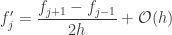
where $\Omega$ is the multiplicity. The remaining quantities of temperature were obtained using a simplified form of the central difference equations for the first order derivative. The respective definitions of temperature and heat capacity are

$\displaystyle T = \frac{\partial U}{\partial S}, (3)$

and

$\displaystyle C_{V} = \frac{\partial U}{\partial T}, (4)$

where $U$ represents the internal energy of the Einstein solid, and $S$ is the entropy. The generalized from of the first order central difference approximation has the form

$\displaystyle \frac{dy_{j}}{dx}\approx \frac{y_{j+1}-y_{j-1}}{2h} + \mathcal{O}(h^{2}), (5)$

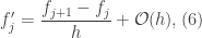
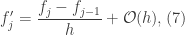
where $\mathcal{O}(h^{2})$ represents the higher order terms, in this case, the quadratic, cubic, quartic, and so on, and $h$ is the step size for each iteration. For the final iteration (when $q = 100$ units), instead of using the central difference approximation, a backward difference approximation was employed since there does not exist data for $q = 101$ units of energy. The backward difference approximation has the form

$\displaystyle \frac{dy_{j}}{dx}\approx \frac{y_{j}-y_{j-1}}{h}+\mathcal{O}(h). (6)$

Table I (Dimensionless Parameters):

*Energy q*	Ω	S/k	kT/ε	C/Nk
0	1	0	0	N/A
1	50	3.912023005	0.27969284	0.121826198
2	1275	7.150701458	0.328336604	0.453606383
3	22100	10.00333289	0.367875021	0.536183525
4	292825	12.58733044	0.402937926	0.593741905
5	3162510	14.96687657	0.43524436	0.637773801
6	28989675	17.18245029	0.465656087	0.673043377
7	231917400	19.26189183	0.494675894	0.702124659
8	1652411475	21.22550156	0.522626028	0.72660015
9	10648873950	23.08871999	0.549726805	0.747522024
10	62828356305	24.86367234	0.576136157	0.765628174
11	3.427E+11	26.56012163	0.601971486	0.781456694
12	1.74206E+12	28.18608885	0.627322615	0.795411957
13	8.30828E+12	29.74827387	0.652259893	0.807805226
14	3.73873E+13	31.25235127	0.676839501	0.818880855
15	1.59519E+14	32.70318415	0.701107048	0.828833859
16	6.48046E+14	34.1049827	0.725100078	0.837822083
17	2.51594E+15	35.4614241	0.748849881	0.845974847
18	9.3649E+15	36.77574496	0.772382808	0.853399232
19	3.35165E+16	38.05081369	0.795721261	0.860184741
20	1.15632E+17	39.28918792	0.818884446	0.866406816
21	3.8544E+17	40.49316072	0.84188895	0.872129523
22	1.24392E+18	41.66479814	0.864749193	0.877407641
23	3.89401E+18	42.80597005	0.887477794	0.882288296
24	1.18443E+19	43.91837566	0.910085848	0.88681226
25	3.5059E+19	45.00356493	0.932583169	0.891014994
26	1.01132E+20	46.0629565	0.954978471	0.89492748
27	2.84667E+20	47.09785298	0.977279528	0.898576916
28	7.82835E+20	48.10945389	0.999493303	0.901987268
29	2.10556E+21	49.09886689	1.021626052	0.905179739
30	5.54463E+21	50.06711736	1.043683421	0.908173155
31	1.43087E+22	51.01515679	1.065670516	0.910984284
32	3.6219E+22	51.94387004	1.087591972	0.913628113
33	8.99987E+22	52.85408172	1.109452006	0.916118071
34	2.19703E+23	53.74656181	1.131254467	0.918466228
35	5.27286E+23	54.62203054	1.153002873	0.920683463
36	1.24498E+24	55.48116286	1.174700452	0.9227796
37	2.89374E+24	56.32459225	1.196350168	0.924763536
38	6.62514E+24	57.1529142	1.217954752	0.926643346
39	1.4949E+25	57.96668937	1.239516722	0.928426373
40	3.32616E+25	58.76644629	1.261038406	0.930119309
41	7.30133E+25	59.55268389	1.282521958	0.931728264
42	1.58195E+26	60.32587378	1.303969378	0.933258829
43	3.38465E+26	61.08646224	1.325382522	0.934716125
44	7.15391E+26	61.8348721	1.346763119	0.936104855
45	1.49437E+27	62.57150439	1.368112778	0.937429341
46	3.08621E+27	63.29673989	1.389433002	0.938693566
47	6.30374E+27	64.01094048	1.410725193	0.9399012
48	1.27388E+28	64.71445045	1.431990666	0.941055635
49	2.54776E+28	65.40759763	1.45323065	0.942160007
50	5.04457E+28	66.09069447	1.4744463	0.943217222
51	9.89131E+28	66.76403902	1.495638697	0.944229971
52	1.9212E+29	67.42791582	1.516808861	0.945200757
53	3.6974E+29	68.08259672	1.537957749	0.946131903
54	7.05244E+29	68.72834166	1.559086264	0.947025573
55	1.33355E+30	69.36539938	1.580195257	0.947883783
56	2.50041E+30	69.99400804	1.60128553	0.948708411
57	4.64989E+30	70.61439586	1.622357843	0.949501213
58	8.57824E+30	71.22678169	1.643412912	0.95026383
59	1.57025E+31	71.83137547	1.664451416	0.950997796
60	2.85263E+31	72.42837879	1.685473998	0.951704548
61	5.14408E+31	73.01798529	1.706481267	0.952385432
62	9.20957E+31	73.60038111	1.7274738	0.953041713
63	1.63726E+32	74.17574525	1.748452147	0.953674575
64	2.89078E+32	74.74424999	1.769416829	0.954285135
65	5.06999E+32	75.30606117	1.79036834	0.95487444
66	8.83407E+32	75.86133855	1.811307153	0.955443478
67	1.52948E+33	76.41023613	1.832233716	0.955993177
68	2.63161E+33	76.95290236	1.853148456	0.956524415
69	4.50043E+33	77.48948048	1.874051781	0.957038017
70	7.65073E+33	78.02010873	1.894944079	0.957534764
71	1.29308E+34	78.54492059	1.915825721	0.958015394
72	2.17309E+34	79.06404502	1.936697061	0.958480604
73	3.63175E+34	79.57760662	1.957558438	0.958931052
74	6.03655E+34	80.08572588	1.978410175	0.959367363
75	9.98043E+34	80.58851934	1.999252581	0.959790129
76	1.64152E+35	81.08609973	2.020085953	0.960199908
77	2.68612E+35	81.57857622	2.040910573	0.960597234
78	4.37356E+35	82.06605448	2.061726714	0.960982609
79	7.08627E+35	82.54863689	2.082534635	0.961356514
80	1.14266E+36	83.02642266	2.103334587	0.961719401
81	1.8339E+36	83.49950796	2.124126809	0.962071705
82	2.92977E+36	83.96798603	2.14491153	0.962413835
83	4.65939E+36	84.43194735	2.165688971	0.962746183
84	7.37736E+36	84.89147968	2.186459344	0.963069122
85	1.16302E+37	85.34666822	2.207222854	0.963383006
86	1.82567E+37	85.7975957	2.227979695	0.963688173
87	2.85392E+37	86.24434247	2.248730056	0.963984945
88	4.44304E+37	86.68698658	2.269474119	0.964273631
89	6.8892E+37	87.12560389	2.290212057	0.964554522
90	1.064E+38	87.56026816	2.31094404	0.9648279
91	1.63692E+38	87.99105107	2.331670228	0.965094032
92	2.50876E+38	88.41802239	2.352390779	0.965353173
93	3.83058E+38	88.84124995	2.373105841	0.965605568
94	5.82737E+38	89.2607998	2.39381556	0.965851451
95	8.83307E+38	89.67673621	2.414520077	0.966091045
96	1.33416E+39	90.08912176	2.435219526	0.966324564
97	2.00812E+39	90.4980174	2.455914037	0.966552213
98	3.01218E+39	90.90348251	2.476603736	0.966774189
99	4.50306E+39	91.30557493	2.497288745	1.287457337
100	6.70955E+39	91.70435105	2.507672727	1.926043463

Graphing the entropy vs. energy, and the heat capacity vs. temperature gives the following:

Graphs I & II

Part II: Let $q = 100$ units and let $N = 5000$ . Using this in the calculation yields the following table for this Einstein solid. This “dilutes” the system and lowers the temperature:

Table II (Dimensionless Parameters):

*Energy q*	Ω	S/k	kT/ε	C/Nk
0	1	0	0	N/A
1	5000	8.517193	0.122388	0.003049
2	12502500	16.34144	0.131206	0.026553
3	2.08E+10	23.76042	0.137453	0.035575
4	2.61E+13	30.89192	0.14245	0.043342
5	2.61E+16	37.80047	0.146681	0.050387
6	2.18E+19	44.52691	0.150388	0.056922
7	1.56E+22	51.09939	0.153709	0.063064
8	9.74E+24	57.53854	0.156731	0.068885
9	5.42E+27	63.86011	0.159515	0.074436
10	2.72E+30	70.07651	0.162105	0.079755
11	1.24E+33	76.19781	0.164531	0.08487
12	5.16E+35	82.23229	0.166818	0.089804
13	1.99E+38	88.18693	0.168985	0.094575
14	7.13E+40	94.06767	0.171047	0.099198
15	2.38E+43	99.87961	0.173017	0.103687
16	7.47E+45	105.6272	0.174905	0.108052
17	2.2E+48	111.3144	0.176719	0.112303
18	6.14E+50	116.9446	0.178467	0.116448
19	1.62E+53	122.5209	0.180154	0.120494
20	4.07E+55	128.0462	0.181787	0.124447
21	9.73E+57	133.5229	0.183368	0.128314
22	2.22E+60	138.9532	0.184904	0.132098
23	4.85E+62	144.3393	0.186396	0.135806
24	1.02E+65	149.683	0.187849	0.13944
25	2.04E+67	154.9861	0.189265	0.143004
26	3.94E+69	160.2502	0.190646	0.146503
27	7.34E+71	165.4768	0.191995	0.149939
28	1.32E+74	170.6671	0.193314	0.153316
29	2.28E+76	175.8226	0.194604	0.156635
30	3.83E+78	180.9444	0.195868	0.159899
31	6.21E+80	186.0336	0.197106	0.16311
32	9.77E+82	191.0912	0.19832	0.166272
33	1.49E+85	196.1183	0.199512	0.169384
34	2.21E+87	201.1157	0.200682	0.172451
35	3.17E+89	206.0843	0.201831	0.175472
36	4.44E+91	211.025	0.202961	0.17845
37	6.04E+93	215.9384	0.204073	0.181387
38	8E+95	220.8254	0.205166	0.184283
39	1.03E+98	225.6866	0.206243	0.18714
40	1.3E+100	230.5227	0.207304	0.18996
41	1.6E+102	235.3343	0.208349	0.192743
42	1.9E+104	240.122	0.209379	0.195491
43	2.3E+106	244.8863	0.210395	0.198205
44	2.6E+108	249.6279	0.211397	0.200885
45	2.9E+110	254.3472	0.212386	0.203533
46	3.2E+112	259.0447	0.213363	0.20615
47	3.4E+114	263.7209	0.214327	0.208736
48	3.6E+116	268.3762	0.215279	0.211293
49	3.7E+118	273.0112	0.21622	0.213821
50	3.7E+120	277.6261	0.21715	0.21632
51	3.7E+122	282.2214	0.218069	0.218793
52	3.6E+124	286.7975	0.218978	0.221238
53	3.4E+126	291.3548	0.219877	0.223658
54	3.2E+128	295.8935	0.220766	0.226052
55	2.9E+130	300.4141	0.221646	0.228422
56	2.7E+132	304.9169	0.222517	0.230768
57	2.4E+134	309.4022	0.22338	0.23309
58	2.1E+136	313.8703	0.224233	0.235388
59	1.8E+138	318.3214	0.225079	0.237665
60	1.5E+140	322.756	0.225917	0.239919
61	1.2E+142	327.1743	0.226746	0.242152
62	1E+144	331.5765	0.227568	0.244363
63	8.1E+145	335.9628	0.228383	0.246555
64	6.4E+147	340.3337	0.229191	0.248725
65	5E+149	344.6892	0.229991	0.250876
66	3.8E+151	349.0296	0.230785	0.253008
67	2.9E+153	353.3553	0.231572	0.255121
68	2.2E+155	357.6663	0.232353	0.257215
69	1.6E+157	361.9629	0.233127	0.259291
70	1.1E+159	366.2453	0.233896	0.261349
71	8.2E+160	370.5137	0.234658	0.263389
72	5.8E+162	374.7683	0.235414	0.265413
73	4E+164	379.0093	0.236165	0.267419
74	2.7E+166	383.237	0.23691	0.269409
75	1.9E+168	387.4514	0.23765	0.271382
76	1.2E+170	391.6527	0.238384	0.273339
77	8.2E+171	395.8412	0.239113	0.275281
78	5.3E+173	400.0169	0.239837	0.277207
79	3.4E+175	404.1802	0.240556	0.279118
80	2.2E+177	408.331	0.24127	0.281015
81	1.4E+179	412.4696	0.24198	0.282896
82	8.4E+180	416.5962	0.242684	0.284763
83	5.2E+182	420.7108	0.243384	0.286616
84	3.1E+184	424.8136	0.24408	0.288455
85	1.9E+186	428.9048	0.244771	0.29028
86	1.1E+188	432.9845	0.245458	0.292092
87	6.5E+189	437.0529	0.24614	0.29389
88	3.7E+191	441.11	0.246819	0.295676
89	2.1E+193	445.156	0.247493	0.297448
90	1.2E+195	449.191	0.248164	0.299208
91	6.7E+196	453.2152	0.24883	0.300955
92	3.7E+198	457.2286	0.249493	0.30269
93	2E+200	461.2315	0.250152	0.304413
94	1.1E+202	465.2238	0.250807	0.306124
95	5.9E+203	469.2057	0.251458	0.307823
96	3.2E+205	473.1774	0.252106	0.30951
97	1.7E+207	477.1389	0.252751	0.311187
98	8.6E+208	481.0903	0.253392	0.312851
99	4.4E+210	485.0318	0.254029	0.418439
100	2.3E+212	488.9634	0.254345	0.628243

Thus the graphs of the entropy vs. energy and heat capacity vs. temperature follow:

Figure 2. Graphs III and IV.

Figure 3. (Figure 1.14 of Schroeder’s Thermal Physics) Heat Capacity curves for Lead (Pb), Aluminum (Al), and Diamond, respectively as a function of temperature in Kelvin.

Graph II shows the prediction for heat capacity as a function of temperature of an Einstein solid for which there are 100 units of energy and 50 oscillators. The data exhibits a trend that appears to reach an asymptote quickly, then when the temperature reaches T ≈ 2.5, there is a sudden increase in the value of the heat capacity. The approach to determining the final data points was switched from a central difference approximation to a backward difference approximation of the last two entries corresponding to energies q = 99 and q = 100 units. If we ignore the last two, the curve approaches an asymptote at C_V = 1. However, the graphs produced are of the dimensionless quantities involved. The overall curve appears to be logarithmic and resembles the heat capacity curve for lead. The initial increase is almost immediate and its slope appears to be slightly less than lead but greater than aluminum.

Graphs III and IV show the prediction for heat capacity in terms of temperature of an Einstein solid for which the energy is the same, but the number of oscillators is now 5000. The temperature has been reduced and the heat capacity vs. temperature yields a graph that shows a trendline that appears linear. Comparing to Figure 3(Fig. 1.14 in the text), this graph resembles the heat capacity curve for diamond. In Figure 3, the diamond curve is linear throughout. The only discrepancies among Graph IV and Figure 3 are the final two data points in Graph IV. Again, a backward difference approximation was used to determine the final data points for this Einstein solid as well. The value for the constant ε was determined by finding the quotient of the entropy and temperature columns and taking the average value of ε for each energy.

This was the numerical analysis of an Einstein solid’s temperature, energy, entropy, and heat capacity. In the next post, I shall discuss the analytical version of this analysis.

Coordinates and Transformations of Coordinates

SOURCES FOR CONTENT: Neuenschwander, D.E., Tensor Calculus for Physics, 2015. Johns Hopkins University Press.

In this post, I continue the introduction of tensor calculus by discussing coordinates and coordinate transformations as applied to relativity theory. (A side note: I have acquired Misner, Thorne, and Wheeler’s Gravitation and will be using it sparingly given its reputation and weight of the material.)

Continue reading Coordinates and Transformations of Coordinates

Derivation of the Finite-Difference Equations

In my final semester, my course load included a graduate course that had two modules: astronomical instrumentation and numerical modeling. The latter focused on developing the equations of motion of geophysical fluid dynamics (See Research in Magnetohydrodynamics). Such equations are then converted into an algorithm based on a specific type of numerical method of solving the exact differential equation.

The purpose of this post is to derive the finite-difference equations. Specifically, I will be deriving the forward, backward, centered first order equations. We start with the Taylor expansion about the points $x_{0}= \pm h$ :

$\displaystyle f(x+h)=\sum_{n=1}^{\infty}\frac{h^{n}}{n!}\frac{d^{n}f}{dx^{n}}, (1)$

and

$\displaystyle f(x-h)=\sum_{n=1}^{\infty}(-1)^{n}\frac{h^{n}}{n!}\frac{d^{n}f}{dx^{n}}. (2)$

Let $f(x_{j})=f_{j}, f(x_{j}+h)=f_{j+1}, f(x_{j}-h)=f_{j-1}$ . Therefore, if we consider the following differences…

$\displaystyle f_{j+1}-f_{j}=f^{\prime}_{j}+f^{\prime \prime}_{j}\frac{h^{2}}{2!}+...+f^{n}_{j}\frac{h^{n}}{n!}, (3)$

and

$\displaystyle f_{j}-f_{j-1}=hf^{\prime}_{j}-\frac{h^{2}}{2!}f^{\prime \prime}_{j}+...\mp \frac{h^{n}}{n!}f^{n}_{j}, (4)$

and

$\displaystyle f_{j+1}-f_{j-1}=2hf^{\prime}_{j}+\frac{2h^{3}}{3!}f^{\prime\prime\prime}_{j}+..\mp \frac{h^{n}}{n!}f^{n}_{j}, (5)$

and if we keep only linear terms, we get

$\displaystyle f^{\prime}_{j}=\frac{f_{j+1}-f_{j}}{h}+\mathcal{O}(h), (6)$

$\displaystyle f^{\prime}_{j}=\frac{f_{j}-f_{j-1}}{h}+\mathcal{O}(h), (7)$

and

$\displaystyle f^{\prime}_{j}=\frac{f_{j+1}-f_{j-1}}{2h}+\mathcal{O}(h)$

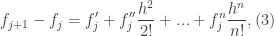
where the first is the forward difference, the second is the backward difference, the last is the centered difference, and $\mathcal{O}(h)$ represents the quadratic, cubic, quartic,quintic,etc. terms. One can use similar logic to derive the second-order finite-difference equations.

Helicity and Magnetic Helicity

SOURCE FOR CONTENT: Davidson, P.A., 2001, An Introduction to Magnetohydrodynamics. 3.

The purpose of this post is to introduce the concepts of helicity as an integral invariant and its magnetic analog. More specifically, I will be showing that

$\displaystyle h = \int_{V_{\omega}}\textbf{u}\cdot \omega d^{3}r (1)$

is invariant and thus correlates to the conservation of vortex line topology using the approach given in the source material above. I will then discuss magnetic helicity and how it relates to MHD.

Consider the total derivative of $\textbf{u}\cdot \omega$ :

$\displaystyle \frac{D}{Dt}(\textbf{u}\cdot \omega) = \frac{D\textbf{u}}{Dt}\cdot \omega + \frac{D\omega}{Dt}\cdot \textbf{u}, (2)$

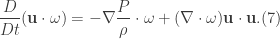
where I have used the product rule for derivatives. Also I denote a total derivative as $\frac{D}{Dt} = \frac{\partial}{\partial t}+(\nabla \cdot \textbf{v})$ so as not to confuse it with the notation for an ordinary derivative. Recall the Navier-Stokes’ equation and the vorticity equation

$\displaystyle \frac{\partial \textbf{u}}{\partial t}+(\nabla \cdot \textbf{v})\textbf{u}=\textbf{F}-\frac{1}{\rho}\nabla P + \nu \nabla^{2}\textbf{u}, (3)$

and

$\displaystyle \frac{\partial \omega}{\partial t}+(\nabla \cdot \textbf{v})\omega =(\nabla \cdot \omega)\textbf{u} +\eta \nabla^{2}\omega (4).$

Let $\textbf{F}=0$ and let $\eta \nabla^{2} \omega \equiv 0$ and $\nu \nabla^{2} \textbf{u} \equiv 0$ . Then,

$\displaystyle \frac{D\textbf{u}}{Dt}=-\nabla \frac{P}{\rho}, (5)$

and

$\displaystyle \frac{D\omega}{Dt}=(\nabla \cdot \omega)\textbf{u}. (6)$

If we substitute Eqs. (5) and (6) into Eq.(2), we get

$\displaystyle \frac{D}{Dt}(\textbf{u}\cdot \omega)=-\nabla \frac{P}{\rho}\cdot \omega + (\nabla \cdot \omega)\textbf{u}\cdot \textbf{u}. (7)$

Evaluating each scalar product gives

$\displaystyle -2\nabla \frac{P}{\rho}\omega + \omega u^{2}\nabla = 0. (8)$

If we divide by 2 and note the definition of the scalar product, we may rewrite this as follows

$\displaystyle \nabla \cdot \bigg\{-\frac{P}{\rho}\omega +\frac{u^{2}}{2}\omega\bigg\}=0. (9)$

With this in mind, consider now the total derivative of $(\textbf{u}\cdot \omega)$ multiplied by a volume element $\delta V$ given by

$\displaystyle \frac{D}{Dt}(\textbf{u}\cdot \omega)\delta V = \nabla \cdot \bigg\{-\frac{P}{\rho}\omega +\frac{u^{2}}{2}\omega\bigg\}\delta V. (10)$

When the above equation is integrated over a volume $V_{\omega}$ , the total derivative becomes an ordinary time derivative. Thus, Eq.(10) becomes

$\displaystyle \int_{V_{\omega}}\frac{d}{dt}(\textbf{u}\cdot \omega)dV=\iint_{S_{\omega}}\bigg\{\nabla \cdot [-\frac{P}{\rho}\omega + \frac{u^{2}}{2}\omega ]\bigg\}\cdot d\textbf{S}=0. (11)$

Hence, Eq.(11) shows that helicity is an integral invariant. In this analysis, we have assumed that the fluid is inviscid. If one considers two vortex lines (as Davidson does as a mathematical example), one finds that there exists two contributions to the overall helicity, corresponding to an individual vortex line. If one considers the vorticity multiplied by a volume element, one finds that for each line, their value helicity is the same. Thus, because they are the same, we can say that the overall helicity remains invariant and hence are linked. If they weren’t linked, then the helicity would be 0. In regards to magnetic helicity we define this as

$\displaystyle h_{m}=\int_{V_{B}}\textbf{A}\cdot \textbf{B}dV, (12)$

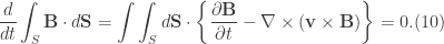
where $\textbf{A}$ is the magnetic vector potential which is described by the following relations

$\displaystyle \nabla \times \textbf{A}=\textbf{B}, (13.1)$

and

$\displaystyle \nabla \cdot \textbf{A}=0. (13.2)$

Again, we see that magnetic helicity is also conserved. However, this conservation arises by means of Alfven’s theorem of flux freezing in which the magnetic field lines manage to preserve their topology.

“Proof” of Alfven’s Theorem of Flux Freezing

SOURCE FOR CONTENT: Choudhuri, A.R., 2010. Astrophysics for Physicists. Ch. 8.

In the previous post we saw the consequences of different regimes of the magnetic Reynolds’ number under which either diffusion or advection of the magnetic field dominates. In this post, I shall be doing a “proof” of Alven’s Theorem of Flux Freezing. (I hesitate to call it a proof since it lacks the mathematical rigor that one associates with a proof.) Also note in this post, I will be working with the assumption of a high magnetic Reynolds number.

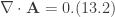
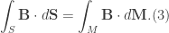
Alfven’s Theorem of Flux Freezing: Suppose we have a surface $S$ located within a plasma at some initial time $t_{0}$ . From the theorem it is known that the flux of the associated magnetic field is linked with surface $S$ by

$\displaystyle \int_{S}\textbf{B}\cdot d\textbf{S}. (1)$

At some later time $t^{\prime}$ , the elements of plasma contained within $S$ at $t_{0}$ move to some other point and will constitute some different surface $M$ . The magnetic flux, linked to $M$ at $t^{\prime}$ by

$\displaystyle \int_{M}\textbf{B}\cdot d\textbf{M}, (2)$

from which we may mathematically state the theorem as

$\displaystyle \int_{S}\textbf{B}\cdot d\textbf{S}=\int_{M}\textbf{B}\cdot d\textbf{M}. (3)$

If we know that the magnetic field evolves in time in accordance to the induction equation we may express Eq.(3) as

$\displaystyle \frac{d}{dt}\int_{S}\textbf{B}\cdot d\textbf{S}=0. (4)$

To confirm that this is true, we note the two ways magnetic flux may change as being due to either (1) some intrinsic variability of the magnetic field strength or (2) movement of the surface. Therefore, either way it follows that

$\displaystyle \frac{d}{dt}\int_{S}\textbf{B}\cdot d\textbf{S}=\int_{S}\frac{\partial \textbf{B}}{\partial t}\cdot d\textbf{S}+\int_{S}\textbf{B}\cdot \frac{d}{dt}(d\textbf{S}). (5)$

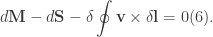
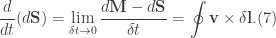
Now, consider again the two surfaces. Let us suppose now that $M$ is displaced some distance relative to $S$ . Further, let us also suppose that this displacement occurs during a time interval $t^{\prime}=t_{0}+\delta t.$ Additionally, if we imagine a cylinder formed by projecting a circular cross-section from one surface to the other, we may consider its length to be $\delta l$ with area given by the cross product: $-\delta t \textbf{v}\times \delta\textbf{l}$ . Moreover, since we know that the area of integration is a closed region we see that the integral vanishes (goes to 0). Thus, we may write the difference

$\displaystyle d\textbf{M}-d\textbf{S}-\delta \oint \textbf{v}\times \delta \textbf{l}=0 (6).$

Recall the definition for a derivative, we may apply it to the second term on the right hand side of Eq.(5) to get

$\displaystyle \frac{d}{dt}(d\textbf{S})=\lim_{\delta t\rightarrow 0}\frac{d\textbf{M}-d\textbf{S}}{\delta t}=\oint \textbf{v}\times \delta \textbf{l}. (7)$

Thus the term becomes

$\displaystyle \int_{S}\textbf{B}\cdot \frac{d}{dt}(d\textbf{S})=\int \oint \textbf{B}\cdot (\textbf{v}\times \delta\textbf{l})=\int \oint (\textbf{B}\times \textbf{v})\cdot \delta l. (8)$

Since the integrals that exist interior to the boundary of the surface (call it path $C$ ) vanish and recall Stokes’ theorem

$\displaystyle \oint_{\partial \Omega}\textbf{F}\cdot d\textbf{r}=\int\int_{\Omega} (\nabla \times \textbf{F})\cdot d\Omega,$

and applying it to Eq.(8) we arrive at

$\displaystyle \frac{d}{dt}\int_{S}\textbf{B}\cdot d\textbf{S}=\oint_{\partial S}(\textbf{B}\times\textbf{v}) \cdot \delta \textbf{l}=\int\int_{S}\bigg\{\nabla \times (\textbf{B}\times\textbf{v})\bigg\}\cdot d\textbf{S}. (9)$

Recall that we are dealing with high magnetic Reynolds number, if we use the corresponding form of the induction equation in Eq.(9) we arrive at

$\displaystyle \frac{d}{dt}\int_{S}\textbf{B}\cdot d\textbf{S}=\int\int_{S}d\textbf{S}\cdot \bigg\{ \frac{\partial \textbf{B}}{\partial t}-\nabla\times (\textbf{v}\times \textbf{B})\bigg\}= 0. (10)$

Thus, this completes the “proof”.

Deriving the Bessel Function of the First Kind for Zeroth Order

NOTE: I verified the solution using the following text: Boyce, W. and DiPrima, R. Elementary Differential Equations.

In this post, I shall be deriving the Bessel function of the first kind for the zeroth order Bessel differential equation. Bessel’s equation is encountered when solving differential equations in cylindrical coordinates and is of the form

$\displaystyle x^{2}\frac{d^{2}y}{dx^{2}}+x\frac{dy}{dx}+(x^{2}-\nu^{2})y(x)=0, (1)$

where $\nu = 0$ describes the order zero of Bessel’s equation. I shall be making use of the assumption

$\displaystyle y(x)=\sum_{j=0}^{\infty}a_{j}x^{j+r}, (2)$

where upon taking the first and second order derivatives gives us

$\displaystyle \frac{dy}{dx}=\sum_{j=0}^{\infty}(j+r)a_{j}x^{j+r-1}, (3)$

and

$\displaystyle \frac{d^{2}y}{dx^{2}}=\sum_{j=0}^{\infty}(j+r)(j+r-1)a_{j}x^{j+r-2}. (4)$

Substitution into Eq.(1) and noting the order of the equation we arrive at

$\displaystyle x^{2}\sum_{j=0}^{\infty}(j+r)(j+r-1)a_{j}x^{j+r-2}+x\sum_{j=0}^{\infty}(j+r)a_{j}x^{j+r-1}+x^{2}\sum_{j=0}^{\infty}a_{j}x^{j+r}=0. (5)$

Distribution and simplification of Eq.(5) yields

$\displaystyle \sum_{j=0}^{\infty}\bigg\{(j+r)(j+r-1)+(j+r)\bigg\}a_{j}x^{j+r}+\sum_{j=0}^{\infty}a_{j}x^{j+r+2}=0. (6)$

If we evaluate the terms in which $j=0$ and $j=1$ , we get the following

$\displaystyle a_{0}\bigg\{r(r-1)+r\bigg\}x^{r}+a_{1}\bigg\{(1+r)r+(1+r)\bigg\}x^{r+1}+\sum_{j=2}^{\infty}\bigg\{[(j+r)(j+r-1)+(j+r)]a_{j}+a_{j-2}\bigg\}x^{j+r}=0, (7)$

where I have introduced the dummy variable $m=(j+r)-2$ and I have shifted the indices downward by 2. Consider now the indicial equation (coefficients of $a_{0}x^{r}$ ),

$\displaystyle r(r-1)+r=0, (8)$

which upon solving gives $r=r_{1}=r_{2}=0$ . We may determine the recurrence relation from summation terms from which we get

$\displaystyle a_{j}(r)=\frac{-a_{j-2}(r)}{[(j+r)(j+r-1)+(j+r)]}=\frac{-a_{j-2}(r)}{(j+r)^{2}}. (9)$

To determine $J_{0}(x)$ we let $r=0$ in which case the recurrence relation becomes

$\displaystyle a_{j}=\frac{-a_{j-2}}{j^{2}}, (10)$

where $j=2,4,6,...$ . Thus we have

$\displaystyle J_{0}(x)=a_{0}x^{0}+a_{1}x+... (11)$

The only way the second term above is 0 is if $a_{1}=0$ . So, the successive terms are $a_{3},a_{5},a_{7},..., = 0$ . Let $j=2k$ , where $k\in \mathbb{Z}^{+}$ , then the recurrence relation is again modified to

$\displaystyle a_{2k}=\frac{-a_{2k-2}}{(2k)^{2}}. (12)$

In general, for any value of $k$ , one finds the expression

$\displaystyle ... \frac{(-1)^{k}a_{0}x^{2k}}{2^{2k}(k!)^{2}}. (13)$

Thus our solution for the Bessel function of the first kind is

$\displaystyle J_{0}(x)=a_{0}\bigg\{1+\sum_{k=1}^{\infty}\frac{(-1)^{k}x^{2k}}{2^{2k}(k!)^{2}}\bigg\}. (14)$

Share this:

Like this:

Share this:

Like this:

Share this:

Like this:

Share this:

Like this:

Share this:

Like this:

Share this:

Like this:

Share this:

Like this:

Share this:

Like this:

Share this:

Like this:

Share this:

Like this: