A PROBLEM IN THERMODYNAMICS AND STATISTICAL MECHANICS: ANALYTICAL AND NUMERICAL STUDY OF AN EINSTEIN SOLID-Analytical Solution

IMAGE CREDIT/OBTAINED FROM: https://mappingignorance.org/2015/12/17/einstein-and-quantum-solids/

Quite some time ago, I had posted a numerical study of an Einstein solid and I now present the analytical study of an Einstein solid. As this was one problem in one of my problem sets while studying thermodynamics and statistical mechanics, one may find this exact problem in the following text:

Schroeder D.V., An Introduction to Thermal Physics, (2000). Addison Wesley Longman. Chapter 3: Interactions and Implications: Problem 3.25. pp. 108.

What I will be presenting is my solution to this problem and I will be offering my interpretation of the problem statement and the implications of the solution.

We begin with the provided approximation,

$\displaystyle \Omega(N,q)\approx \bigg(\frac{q+N}{q}\bigg)^{q}\bigg(\frac{q+N}{N}\bigg)^{N}. (1)$

This expression represents the multiplicity of an Einstein solid with $N$ oscillators and $q$ energy units. Recall that the equation to find the entropy is the following

$\displaystyle S=k\ln{(\Omega(N,q))}. (2)$

Thus, upon substitution of the multiplicity (Eq.(1)) into the equation for entropy (Eq.(2)), one arrives at the equation

$\displaystyle S=k\ln{\bigg\{\bigg(\frac{q+N}{q}\bigg)^{q}\bigg(\frac{q+N}{N}\bigg)^{N}\bigg\}}. (3)$

Upon making use of the properties of logarithms, we may write the equation equivalently as

$\displaystyle S = k\ln{\bigg\{\bigg(\frac{q+N}{q}\bigg)^{q}\bigg\}}+k\ln{\bigg\{(\frac{q+N}{N}\bigg)^{N}\bigg\}}, (4)$

and again using the well-known property that $\ln{x}^{a}=a\ln{x}$ , we may further simplify Eq.(4) such that we arrive at the expression for the entropy of an Einstein solid:

$\displaystyle S = kq\ln{\bigg\{\bigg(\frac{q+N}{q}\bigg)\bigg\}}+Nk\ln{\bigg\{\bigg(\frac{q+N}{N}\bigg)\bigg\}}. (5)$

We may omit the factor of $(2\pi q(q+N))^{1/2}N^{-1/2}$ from Stirling’s approximation owing to the fact that if $N$ and $q$ are very large numbers, then $\sqrt{q}<<q$ and $\sqrt{N}<<N$ . Hence, it follows that $\sqrt{q+N}<<(q+N)$ . So we see that the aforementioned factor is of no consequence provided that $q$ and $N$ (i.e. the number of energy units and oscillators) is very large.

The second part of this problem asks to take the expression we derived for the entropy and compute the temperature. Recall that the definition for temperature is given by the equation

$\displaystyle \frac{1}{T}=\bigg(\frac{\partial S}{\partial U}\bigg)^{-1}. (6)$

From substitution we may write the following

$\displaystyle \frac{1}{T}=\bigg\{\frac{\partial}{\partial U}\bigg(k\bigg(\frac{U}{\epsilon}+N\bigg)\ln{\bigg(\frac{U}{\epsilon}+N\bigg)}\bigg)-\frac{\partial}{\partial U}\bigg(\frac{kU}{\epsilon}\ln{\bigg(\frac{U}{\epsilon}\bigg)}\bigg)-\frac{\partial}{\partial U} (N\ln{(N))}\bigg\}^{-1}, (7)$

where I have made use of the properties of logarithms and made the substitution $q=U/\epsilon$ . Differentiating and simplifying yields,

$\displaystyle \frac{1}{T}=\bigg\{\bigg(\frac{k}{\epsilon}\bigg)\ln{\bigg(\frac{U}{\epsilon}+N\bigg)}-\ln{\bigg(\frac{U}{\epsilon}\bigg)}\bigg\}^{-1}. (8)$

Further simplification yields the equation for temperature $T$ of an Einstein solid

$\displaystyle T = \frac{\epsilon}{k\ln{\bigg(\frac{U+\epsilon N}{U}}\bigg)}. (9)$

Part three asks us to find the equation for the heat capacity from our temperature equation. Recall that the equation for heat capacity is of the form

$\displaystyle C = \bigg(\frac{\partial U}{\partial T}\bigg). (10)$

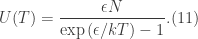
However, we need an equation for the internal energy $U$ as a function of temperature $T$ . We actually have the opposite. So we must solve Eq.(9) for the internal energy, and doing so yields

$\displaystyle U(T)=\frac{\epsilon N}{\exp{(\epsilon/kT)}-1}. (11)$

Substituting Eq.(11) into Eq.(10) gives

$\displaystyle C = \bigg(\frac{\partial U}{\partial T}\bigg)=\frac{\partial}{\partial T}\bigg(\frac{\epsilon N}{\exp{(\epsilon/kT)}-1}\bigg). (12)$

Using the quotient rule for derivatives gives the equation for the heat capacity

$\displaystyle C =\bigg(\frac{\epsilon^{2}N}{kT^{2}}\bigg) \bigg(\frac{\exp{(\epsilon/kT)}}{{(\exp{(\epsilon/kT)}-1)}^{2}}\bigg). (13)$

The next part asked to show that in the limit $T \rightarrow \infty$ , the heat capacity $C =Nk$ . Recall that the Taylor series expansion for the exponential function $\exp{(x)}$ is given by

$\displaystyle \exp{(x)}=\sum_{j=0}^{\infty}\frac{x^{j}}{j!}. (14)$

For small values of $x$ we may make the approximation $\exp{(x)}\approx 1+ x$ . Then we have the approximate relation

$\displaystyle C \approx \frac{\epsilon^{2}N}{kT^{2}}\frac{(1+\epsilon/kT)}{(1+(\epsilon/kT)-1)^{2}}=\frac{\epsilon^{2}N(1+(\epsilon/kT))}{kT^{2}(\epsilon^{2}/k^2 T^2)}= Nk(1+(\epsilon/kT)). (15)$

Then considering the aforementioned limit yields

$\displaystyle \lim_{T \rightarrow \infty} C = \lim_{T \rightarrow \infty} \bigg(Nk(1+(\epsilon/kT))\bigg)= Nk. (16)$

The final part of my solution to this problem (I did not complete the last portion of the problem see the aforementioned reference for the problem) asks us to graph the resultant equation relating the heat capacity and the temperature. Below is a plot of the function in the technical computing software Maple.

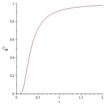
Fig.1 Heat Capacity vs. Temperature

For low temperatures, the heat capacity initially starts at $0$ . However, when $t=0.097$ , there appears to be a dramatic increase in the heat capacity in the dimensionless quantity $C/Nk$ . If the heat capacity $C$ is graphed as a function of temperature $T$ , and one uses the $\epsilon$ values for each of the lead and aluminum curves produced in Fig. 1.14 of Schroeder’s An Introduction to Thermal Physics.