Coordinates and Transformations of Coordinates

SOURCES FOR CONTENT: Neuenschwander, D.E., Tensor Calculus for Physics, 2015. Johns Hopkins University Press.

In this post, I continue the introduction of tensor calculus by discussing coordinates and coordinate transformations as applied to relativity theory. (A side note: I have acquired Misner, Thorne, and Wheeler’s Gravitation and will be using it sparingly given its reputation and weight of the material.)

In relativity, one speaks of a point or location in spacetime as an event. An event has 4 coordinates: $x, y, z, t$ . Three spatial and one time coordinate. There are various conventions when writing metrics regarding the time coordinate (e.g. the convention for which $h=c=1$ ). I will not be making that assumption, I will be using the canonical values of Planck’s constant and the speed of light.

Returning from that digression, a more compact manner in which to represent an event would be to assert the following: let the spatial coordinates $x, y, z$ be denoted by $x^{1}, x^{2}, x^{3}$ , and the time coordinate be $x^{0}$ . In general, we can denote the event in spacetime $x^{\mu}$ where $\mu \in \mathbb{Z}^{\pm}$ and I define (I must admit that this definition of a set of integers may not be the most mathematically formal, forgive me) of $\mathbb{Z}^{\pm}= \big\{{x \in \mathbb{Z}|x \geq 0}\big\}$ . Another commonly used name for this is a four-position.
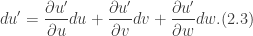
Suppose we have the following expression:

$\displaystyle u^{\prime}=u\cos{(\theta)}+v\sin{(\theta)}, (1)$

If we take the partial derivative of $u^{\prime}$ with respect to $u$ and $v$ , we get

$\displaystyle \frac{\partial u^{\prime}}{\partial u}=\cos{(\theta)}, (2.1)$

and

$\displaystyle \frac{\partial u^{\prime}}{\partial v}=\sin{(\theta)}. (2.2)$

A simple substitution into Eq.(1) yields,

$\displaystyle du^{\prime}=\frac{\partial u^{\prime}}{\partial u}du+\frac{\partial u^{\prime}}{\partial v}dv+\frac{\partial u^{\prime}}{\partial w}dw. (2.3)$

Thus we can see that vectors and their coordinates transform by means of differentials. Hence, if we are located in a coordinate system (call it $S$ ) and we wish to determine our location in a different coordinate system (call that one $S^{\prime}$ ), one of the ways to do that would be using coordinate differentials. Moreover, in many fields of physics, most especially in the realm of fluid mechanics, one regards the components $u = x^{1}, v = x^{2}, w = x^{3}$ . So, by that logic we can state, in general, the transformation rule of vectors as

$\displaystyle dx^{\prime \mu} = \sum_{\nu}\frac{\partial x^{\prime \mu}}{\partial x^{\nu}}dx^{\nu}, (3)$

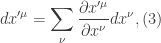
where the indices $\mu, \nu$ represent the integers $0,1,2,3$ .
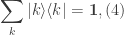
Alternatively, instead of coordinate differentials, one can also use the concepts of matrices to transform a vector $|u\rangle$ from one basis to another, yielding a different vector within a different basis $|u^{\prime}\rangle$ . Recall that the completeness relation is given by

$\displaystyle \sum_{k}|k\rangle \langle k|=\textbf{1}, (4)$

and

$\displaystyle \sum_{\lambda} |\lambda\rangle \langle \lambda|=\textbf{1}. (5)$

I am using $\lambda$ since $\mu$ in the previous post of this series would be confused with the $\mu$ previously defined in this one. Let us multiply by $|u\rangle$ :

$\displaystyle |u\rangle = \textbf{1}|u\rangle = \sum_{k}|k\rangle \langle k|u\rangle = \sum_{k}u^{k}|k\rangle,$

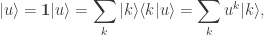
Now multiply by $|\lambda \rangle$ :

$\displaystyle \langle \lambda |u \rangle = \sum_{k} \langle \lambda |k \rangle u^{k}. (6)$

To avoid “tunnel-vision”, the purpose of all this math is to relate the two presentations of coordinate transformations of vectors. The first is the one someone would expect; it involves derivatives, and so, change is inherent in the equation. The latter is much more mathematically elegant and formal, making use of Dirac notation but is, in essence, an equivalent way of saying the same thing.

Share this:

Like this:

Related

Leave a Reply Cancel reply