While I was an undergraduate, one of my smaller research projects involved observing the variable star W Ursae Majoris.
In general, there are six types of binary star systems: Optical double, Visual binary, Astrometric binary, Eclipsing binary, Spectrum binary, and Spectroscopic binary.
In this project, my classmate and I were interested in the eclipsing binary (EW) W Ursae Majoris. An eclipsing binary is a binary system in which one of the stars will pass in front of its companion, effectively causing an eclipse. We are able to observe this by way of generating the light curves of the system. An example light curve is shown below:

(Image was obtained at the URL: https://imagine.gsfc.nasa.gov/educators/hera_college/binary-model.html)
The graph shows a plot of intensity over time (which in this case is an orbital period). Observations of an EW should show dips in the intensity of the two stars. What is really fascinating to me is that we can gain valuable information from this graph. For example, the length of a dip can indicate the masses of the star. If we have a star of mass  and the other is
  such that
  , and if the duration of the decrease in intensity of the system is significant we can then infer that the mass passing in front of its companion is that of . By default, the mass that is being “eclipsed” is . Conversely, if the intensity decreases but only for a short while, the positions are reversed, with passing in front (relatively speaking) and is being “eclipsed”. (I am assuming that the barycenter (i.e. the system’s center of mass) is equidistant from the centers of the two stars.)
Another form of classification of binary stars is whether or not the binary system components are touching or not. More precisely, there are three kinds of close binaries: detached, semi-detached, and contact binary. There are sub-categories of contact binaries: near contact, contact, overcontact, and double contact.
An equipotential surface map of a system (assuming that the binary system has a mass ratio of 2:1, which may be incorrect as most W UMa binaries have a mass ratio of 10:1) is shown below:

Image Credit: Fig.1 of Terrell, D., Eclipsing Binary Stars: Past, Present, and Future. JAAVSO Vol. 30, 2001.
To quickly elaborate, each type of contact binary will fill its inner Lagrangian surface (aka Roche lobes) to an extent. In the context of our project, W Ursae Majoris is an overcontact eclipsing binary system. This type of binary will overfill its inner Lagrangian surface. As a result of this, processes such as mass transfer and accretion can occur. The diagram below shows the orbital evolution of a W UMa EW AC Bootis (in addition to being its own binary system, W UMa is also a class of close binaries)

Image Credit: Fig. 15 of Alton, K., A Unified Roche-Model Light Curve Solution for the W UMa Binary AC Bootis. JAAVSO. Vol. 38, 2010.
The objective of the project was to image the eclipsing binary, measure the apparent magnitude, to process the images, and to obtain a light curve. To observe this system, a classmate and I made use of the 20″ Ritchey-Chrétien telescope at the university observatory. We made use of the CCD camera attached and set a sequence of images to be taken every two minutes. W UMa has a period of approximately 8 hours, however, due to time constraints (and as much as I would have liked to, the weather was not conducive for observations exceeding two hours), we ended up only taking images for around two hours.
After the session was over, we ended up taking a total of roughly 40-50 images. Additionally, the software used to capture the images simultaneously measured the magnitude of W UMa at the time each image was taken. This allowed us to use Excel (and later on MATLAB) to obtain a partial light curve. However, since this is a partial light curve, we can say that an eclipse (and a short one at that) occurs, yet we cannot determine whether or not the local minimum depicted in the graph below is a primary or a secondary minimum–we simply do not have enough data.
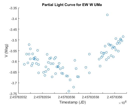
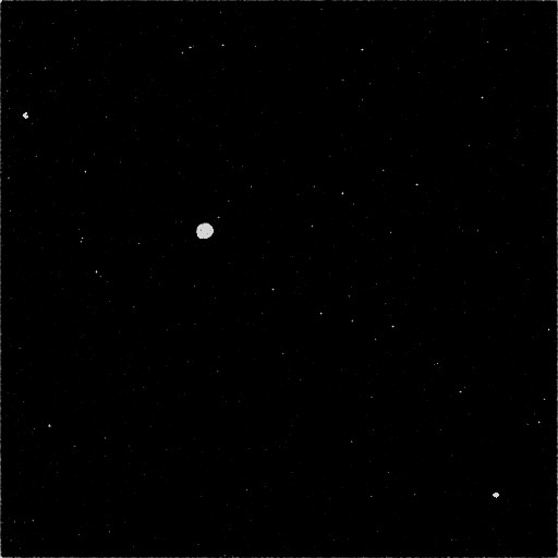
In addition to the partial light curve above, we were able to process the images (using Registax v.6). Below is a stacked image of W UMa. The big blob near the center of the image is the binary. The binary is not able to be resolved by telescopes component-wise.
References:
Caroll, B.W., and Ostlie, D. A., Introduction to Modern Astrophysics. 2017. Cambridge University Press. 7.
Catalog and Atlas of Eclipsing Binaries (CALEB): Types of Binary Stars
http://www.daviddarling.info/encyclopedia/C/close_binary.html
American Association of Variable Star Observers (AAVSO) URL: https://www.aavso.org/vsots_wuma
Journal of American Association of Variable Star Observers: Figure References


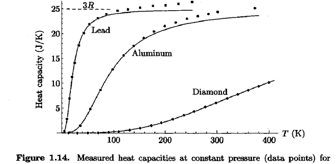
 …The model of a solid as a collection of identical oscillators with quantized energy units…”
 for each of those solids.”
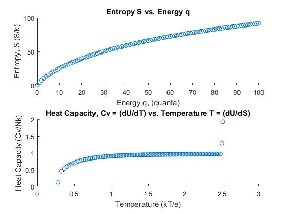
 units, and let $N = 50$. The corresponding data table for this Einstein solid follows. The following set of equations were used to determine the multiplicity and entropy.

 is the multiplicity. The remaining quantities of temperature were obtained using a simplified form of the central difference equations for the first order derivative. The respective definitions of temperature and heat capacity are

 represents the internal energy of the Einstein solid, and
  is the entropy. The generalized from of the first order central difference approximation has the form
 represents the higher order terms, in this case, the quadratic, cubic, quartic, and so on, and
  is the step size for each iteration. For the final iteration (when
  units of energy. The backward difference approximation has the form
 . Using this in the calculation yields the following table for this Einstein solid. This “dilutes” the system and lowers the temperature:
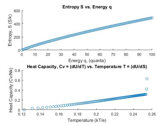

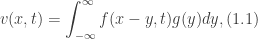
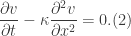
 has finite support and also satisfies the PDE
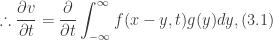


 . This means that
 does satisfy the given PDE (Eq.(2)).
 :
:

 . Therefore, if we consider the following differences…


 represents the quadratic, cubic, quartic,quintic,etc. terms. One can use similar logic to derive the second-order finite-difference equations.

 :
:
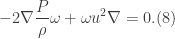
 so as not to confuse it with the notation for an ordinary derivative. Recall the Navier-Stokes’ equation and the vorticity equation

 and let
  and
and  . Then,


 multiplied by a volume element
  given by
 , the total derivative becomes an ordinary time derivative. Thus, Eq.(10) becomes
![\displaystyle \int_{V_{\omega}}\frac{d}{dt}(\textbf{u}\cdot \omega)dV=\iint_{S_{\omega}}\bigg\{\nabla \cdot [-\frac{P}{\rho}\omega + \frac{u^{2}}{2}\omega ]\bigg\}\cdot d\textbf{S}=0. (11)](https://s0.wp.com/latex.php?latex=%5Cdisplaystyle+%5Cint_%7BV_%7B%5Comega%7D%7D%5Cfrac%7Bd%7D%7Bdt%7D%28%5Ctextbf%7Bu%7D%5Ccdot+%5Comega%29dV%3D%5Ciint_%7BS_%7B%5Comega%7D%7D%5Cbigg%5C%7B%5Cnabla+%5Ccdot+%5B-%5Cfrac%7BP%7D%7B%5Crho%7D%5Comega+%2B+%5Cfrac%7Bu%5E%7B2%7D%7D%7B2%7D%5Comega+%5D%5Cbigg%5C%7D%5Ccdot+d%5Ctextbf%7BS%7D%3D0.+%2811%29&bg=ffffff&fg=333333&s=0&c=20201002)

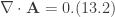
 is the magnetic vector potential which is described by the following relations
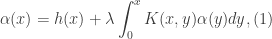
![y\in [0,x]](https://s0.wp.com/latex.php?latex=y%5Cin+%5B0%2Cx%5D&bg=ffffff&fg=333333&s=0&c=20201002) . The first term of the integrand
. The first term of the integrand  denotes the kernel. The kernel of the integral arises from its conversion from an initial value problem. Indeed, solving the integral equation is equivalent to solving the initial value problem of a differential equation. The integral equation includes the initial conditions instead of being added in near the end of the solution of an IVP.
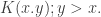
 Then the next iteration of
  is
is
 is
is


 is determined, we may determine the exact solution
  via
via
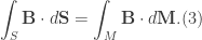
 . From the theorem it is known that the flux of the associated magnetic field is linked with surface
 , the elements of plasma contained within

 Additionally, if we imagine a cylinder formed by projecting a circular cross-section from one surface to the other, we may consider its length to be
  with area given by the cross product:
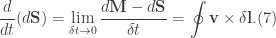
  . Moreover, since we know that the area of integration is a closed region we see that the integral vanishes (goes to 0). Thus, we may write the difference
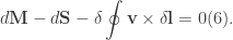

 ) vanish and recall Stokes’ theorem