
If you recall, there was a post I uploaded some time ago where I talked about manifolds and coordinates as a part of my Basics of Tensor Calculus series. I also noted that the post was incomplete. I now plan to rectify that post by treating manifolds properly in this one. The objective of this post is as follows:
- Introduce some basic concepts about topology; in particular, the concept of a homeomorphism is of crucial importance.
- Discuss some prerequisite material from multivariable calculus (e.g. diffeomorphisms and smooth functions).
- Define what is called an
-dimensional differentiable manifold and provide some remarks on the definitions presented.
Part I. Elementary Concepts in Topology:
As I’ve not talked about what a topology is on this blog, I will try to give a quick idea of what a topology of a set is and from there construct the idea of a topological space from which I define a continuous function between two topological spaces which then leads us to the concept of a homeomorphism.
Therefore, we have the following definition:
Definition. (Topology; Topological Space.) Let 

-
;
where
are open in
.
The coordinate pair 
What this definition tells us first is that if we are given a set
We now make a few further definitions related to topological spaces: that of neighborhoods, Hausdorff spaces, closure, interior, and boundary.
Definition. (Closed Set; Closure; Interior; Boundary.) Let 


We now define the concepts of neighborhoods and Hausdorff spaces:
Definition. (Neighborhood; Hausdorff Spaces.) Let 


Now, let 


Definition. (Homeomorphism.) Let 


Part II. Smoothness and Diffeomorphisms
Definition. (Smooth Function.) Let 


Definition. (Diffeomorphism.) Let us consider two open sets 

Part III. Smooth Manifolds
We now come to the purpose of the post: the definition of a manifold.
Definition. (


- For every coordinate map
,
defines a homeomorphism to
. In other words,
is homeomorphic to
- Given two overlapping coordinate patches
with coordinate maps
, respectively, said coordinate maps are compatible in the sense that
and forms a diffeomorphism.
The two conditions stated above can be difficult to process as presented. To provide a more inuitive way of thinking about it, we note that the first condition, in particular, essentially defines the notion of a manifold being locally Euclidean. Rather, if a coordinate patch (or coordinate neighborhood) is selected on the manifold, then there exists a way to assign Euclidean coordinates to that patch in the usual way. Finally, we have defined manifolds with a notion of differentiability, but it is worthy to note that we can easily define an
This post took awhile but I’m hoping to continue to post on some of the topics I’ve been researching recently. The next post (whenever I am able to get to it) will likely consider further topics in manifolds and perhaps some elementary homology theory. Until then, clear skies!
__________________________________________________________________________________________________________________________________________________________________
[References used to study these topics: Manifolds, Tensors, and Forms: An Introduction for Mathematicians and Physicists. Paul Renteln. Ch 3. & A Short Course in Differential Topology. Bjorn Ian Dundas. Ch.2 ]
 and
and  spaces: This section will discuss the concept of a norm as it relates to the spaces
  which take one of the following forms:
 ![[a,b] := \{x\in \mathbb{R}|a\leq x \leq b\} \label{(1.1)}](https://s0.wp.com/latex.php?latex=%5Ba%2Cb%5D+%3A%3D+%5C%7Bx%5Cin+%5Cmathbb%7BR%7D%7Ca%5Cleq+x+%5Cleq+b%5C%7D+%5Clabel%7B%281.1%29%7D&bg=ffffff&fg=333333&s=0&c=20201002) ;
; ;
;![(a,b] := \{x\in \mathbb{R}|a< x\leq b\} \label{(1.3)}](https://s0.wp.com/latex.php?latex=%28a%2Cb%5D+%3A%3D++%5C%7Bx%5Cin+%5Cmathbb%7BR%7D%7Ca%3C+x%5Cleq+b%5C%7D+%5Clabel%7B%281.3%29%7D&bg=ffffff&fg=333333&s=0&c=20201002) ;
; ,
,![I=[a,b]](https://s0.wp.com/latex.php?latex=I%3D%5Ba%2Cb%5D&bg=ffffff&fg=333333&s=0&c=20201002) denoted
denoted  . For dimensions
  , we define the measure of such sets as equalling the
  -times Cartesian product of intervals
  ; that is,
 such that
 is
is  -th
-th  we replace rectangles with cubes and the area with the volume. For dimensions
  , we replace cubes with boxes of
  , denoted
  to be
to be 
 to be a set whose measure
  ; that is, its measure is equal to the outer measure.
  where
where  is the
  -algebra of Lebesgue measurable subsets of
 such that every open ball centered on
  .
.  be a metric space with the defined metric
  . Then an open cover for
  such that
  .
. may be of infinite cardinality.
  , and let
  . Then
  is a limit point or a cluster point of
  , of a subset
  .
. and let
  Then the open interval
  is not a compact set. To see why consider the set of open subsets
  for
for  . Note that
  . However,
  . In other words, (or rather in words) what this says is that if we consider all of the open sets of the form
  contains the interval
  . However, note that if we take only a finite number
  , for simplicity say
  , then we have that the union
  does not contain all of the points that are contained in
  is compact if every sequence in
  that equipped with an inner product
  .
.  where
where  . A point
  is called a limit of the sequence of points if for any
  , there exists
  such that if
  ,
, . If such a limit exists, then we say that the sequence of points
  .
.  which corresponds to the point
  in the metric space
  . We can regard the term
  .
.  of each other in the metric space
  is a complete metric space. Intuitively, what this means is that given a Cauchy sequence that converges in
  .
.  . This serves as the basis for the intuitive concept of a “space”, and our ability to ascribe a distance between to points in three-dimensional space can be described by a distance function
  , or a metric. The underlying set
  a real number
  such that


 and the metric coupled with this set is defined by
  . To verify that this indeed a metric space we must show that the four axioms are satisfied.
  in which
  is defined by
  . Then by definition of
  , so that axiom 1 is satisfied. Suppose now that the points in
  . Then by definition of
  Conversely, suppose that
  By the triangle inequality we have that
  This implies that
  . Thus, condition (2.) is satisfied and hence the distance between two points in
  . By virtue of the definition of the absolute value, we can say that
 , then the distance function between the points
  becomes
 ,
,

 is a non-empty set equipped with a single binary operation
  that satisfies the following four axioms:
 ,
,  ;
; ,
,  ;
; , there exists an element
  ;
; such that
 (we’ll discuss what this notation means later on in the post). Let
  and let
  . We can add these two integers to get another integer, call it
  . This is what we mean by a binary operation.
 , if
, if  is also in the set, then we say that the set is closed under the operation
  . Statement 2 says that given any three elements in the set, the order in which the operation is performed, as dictated by the parentheses, is immaterial. This statement ensures that the elements of the set are associative. To clarify this a bit more, consider the following sum in
  :
:
 . For multiplication, the inverse element is the multiplicative inverse, in which case we have that for every element
  . In the definition, I was careful to include both the right and left inverse. The reason for this is not all sets of elements commute, that is it is not always true that
  . As an example, let
  be the set of all
  matrices whose determinant is non-zero. Matrices are known to non-commutative, and so
  . If it is true that every element in the group commutes, then
  . For addition, the identity element is
  , since given any element of
  , and in multplicative notation
  , depending on the operation involved. If all four of these axioms, as we call them, are satisfied, then the set is a group under the prescribed operation.
 , and the complex numbers
  to name a few. We denote the structure by stating what set we are considering, followed by a the binary operation, written as
  .
. in detail and I will show how to prove that the reals and integers are groups under addition and that the complex numbers are a group under complex multiplication.

 oscillators and
  energy units. Recall that the equation to find the entropy is the following


 , we may further simplify Eq.(4) such that we arrive at the expression for the entropy of an Einstein solid:
 from Stirling’s approximation owing to the fact that if
  and
and  . Hence, it follows that
  . So we see that the aforementioned factor is of no consequence provided that

 . Differentiating and simplifying yields,
 of an Einstein solid

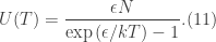


 , the heat capacity
  . Recall that the Taylor series expansion for the exponential function
  is given by
 . Then we have the approximate relation

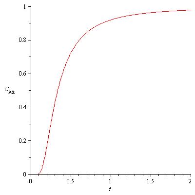
 , there appears to be a dramatic increase in the heat capacity in the dimensionless quantity
  . If the heat capacity
  is graphed as a function of temperature
 is invariant with respect to Lorentz transformations. This is a pretty standard problem in most GR textbooks and in fact in some introductory books on SR.
 , there exists points whose difference relative to
  .
. -dimensional hypersphere whose surface area is given by
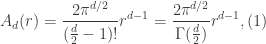
 is the gamma function given by

 . By the method used in a previous section of the aforementioned text, we may write

 , and introducing a variational parameter


 with respect to


 . Since
  for any