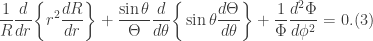
This post deals with the familiar (to the physics student) Laplace’s equation. I am solving this equation in the context of physics, instead of a pure mathematical perspective. This problem is considered most extensively in the context of electrostatics. This equation is usually considered in the spherical polar coordinate system. A lot of finer details are also considered in a mathematical physics course where the topic of spherical harmonics is discussed. Assuming spherical-polar coordinates, Laplace’s equation is

Suppose that the function 


Furthermore, we can separate further the term 

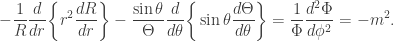
Bringing the radial and angular component to the other side of the equation and setting the azimuthal component equal to a separation constant 
Solving the right-hand side of the equation we get

Now, we set the azimuthal component equal to 
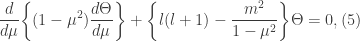
where I have let 

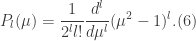
However, the solutions to Eq.(5) are the associated Legendre functions, not polynomials. Therefore, we use the following to determine the associated Legendre functions from the Legendre polynomials:
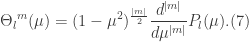
For real solutions 

Now we turn to the radial part which upon substitution of 
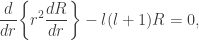
and if we evaluate the derivatives in the first term we get an Euler equation of the form
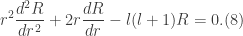
Let us assume that the solution can be represented as

Taking the necessary derivatives and substituting into Eq.(8) gives
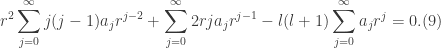
Simplifying the powers of r we find that
![\displaystyle \sum_{j=0}^{\infty}[j(j-1)+2j-l(l+1)]a_{j}r^{j}=0.](https://s0.wp.com/latex.php?latex=%5Cdisplaystyle+%5Csum_%7Bj%3D0%7D%5E%7B%5Cinfty%7D%5Bj%28j-1%29%2B2j-l%28l%2B1%29%5Da_%7Bj%7Dr%5E%7Bj%7D%3D0.&bg=ffffff&fg=333333&s=0&c=20201002)
Now, since 

We can simplify this further to get

Factoring out 

Since this must be true for all values of l, the solution therefore becomes
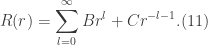
Thus, we can write the solution to Laplace’s equation as
![\displaystyle \psi(r,\theta,\phi) = \sum_{l=0}^{\infty} \sum_{m=0}^{\infty}[Br^{l}+Cr^{-l-1}]\Theta_{l}^{m}(\mu)A\exp({im\phi}), (12)](https://s0.wp.com/latex.php?latex=%5Cdisplaystyle+%5Cpsi%28r%2C%5Ctheta%2C%5Cphi%29+%3D+%5Csum_%7Bl%3D0%7D%5E%7B%5Cinfty%7D+%5Csum_%7Bm%3D0%7D%5E%7B%5Cinfty%7D%5BBr%5E%7Bl%7D%2BCr%5E%7B-l-1%7D%5D%5CTheta_%7Bl%7D%5E%7Bm%7D%28%5Cmu%29A%5Cexp%28%7Bim%5Cphi%7D%29%2C%C2%A0+%2812%29&bg=ffffff&fg=333333&s=0&c=20201002)
for real solutions, and
![\displaystyle \psi(r,\theta,\phi)=\sum_{l=0}^{\infty}\sum_{m=-l}^{l}[Br^{l}+Cr^{-l-1}]\Theta_{l}^{m}(\mu)A\exp({im\phi}), (13)](https://s0.wp.com/latex.php?latex=%5Cdisplaystyle+%5Cpsi%28r%2C%5Ctheta%2C%5Cphi%29%3D%5Csum_%7Bl%3D0%7D%5E%7B%5Cinfty%7D%5Csum_%7Bm%3D-l%7D%5E%7Bl%7D%5BBr%5E%7Bl%7D%2BCr%5E%7B-l-1%7D%5D%5CTheta_%7Bl%7D%5E%7Bm%7D%28%5Cmu%29A%5Cexp%28%7Bim%5Cphi%7D%29%2C+%2813%29&bg=ffffff&fg=333333&s=0&c=20201002)
for complex solutions.

How did you factor j + l out of j^2 + l^2 + j + l = 0?
(j + l)(j + l + 1) = j^2 + l^2 + j + l + 2jl
LikeLiked by 1 person
Hello, thanks for pointing that out. It looks like I made a few sign mistakes that carried through to the values of j. I have updated my solution with my correction.
LikeLike
for some reason my l’s look like larger 1’s…
LikeLiked by 1 person