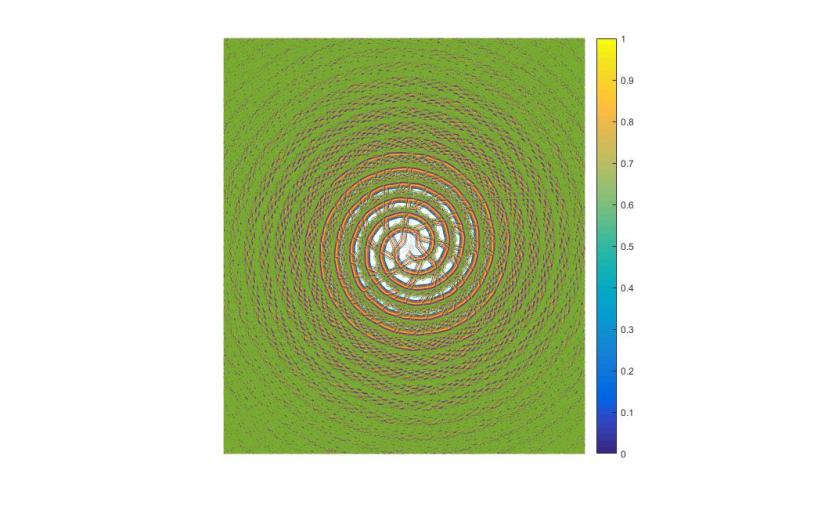
FEATURED IMAGE: This is one of the plots that I will be explaining in Post IV. This plot represents the radiation flux emanating from the primary and secondary components of the system considered.
I realize I haven’t posted anything new recently. This is because I have been working on finishing the research project that I worked on during my final semester as an undergraduate.
However, I now intend to share the project on this blog. I will be starting a series of posts in which I will attempt to explain my project and the results I have obtained and open up a dialogue as to any improvements and/or questions that you may have.
Here is the basic overview of the series and projected content:
Post I: Project Overview:
In this first post, I will introduce the project. I will describe the goals of the project and, in particular, I will describe the nature of the system considered. I will also give a list of references used and mention any and all acknowledgements.
Posts II & III: Radiative Transfer Theory
These posts will most likely be the bulk of the concepts used in the project. I will be defining the quantities used in the research, developing the radiative transfer equation, formulating the problems of radiative transfer, and using the more elementary methods to solving the radiative transfer equation.
Post IV: Monte Carlo Simulations
This post will largely be concerned with the mathematics and physics of Monte Carlo simulations both in the context of probability theory and Ising models. I will describe both and explain how it applies to Monte Carlo simulations of Radiative Transfer.
Post V: Results
I will discuss the results that the simulations produced and explain the data displayed in the posts. I will then discuss the conclusions that I have made and I will also explain the shortcomings of the methods used to produce the results I obtained. I will then open it up to questions or suggestions.
 :
:


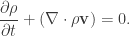
 is
is  . Thus, the integral of the mass flux is
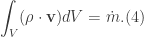


 to be the curl of the fluid velocity:
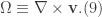
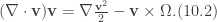
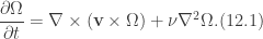

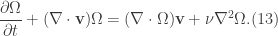
 . Substitution into the continuity equation yields the following
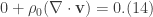
 . Now, since
  , this then means that


 , which means that the charge density must be zero, and we also let the current density
  . Moreover, note that the form of the wave equation as
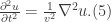


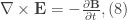
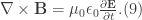
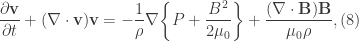
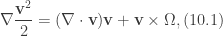
 . Now, take the curl of Eqs.(8) and (9), and we get
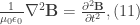
![\frac{1}{c^{2}}=\frac{1}{\mu_{0}\epsilon_{0}} \implies c=\sqrt[]{\mu_{0}\epsilon_{0}}, (12)](https://s0.wp.com/latex.php?latex=%5Cfrac%7B1%7D%7Bc%5E%7B2%7D%7D%3D%5Cfrac%7B1%7D%7B%5Cmu_%7B0%7D%5Cepsilon_%7B0%7D%7D+%5Cimplies+c%3D%5Csqrt%5B%5D%7B%5Cmu_%7B0%7D%5Cepsilon_%7B0%7D%7D%2C+%2812%29&bg=ffffff&fg=333333&s=0&c=20201002)
 is the permeability of free space and
  is the permittivity of free space.
![\delta t = \frac{\delta t_{0}}{\sqrt[]{1-v^{2}/c^{2}}}, (13)](https://s0.wp.com/latex.php?latex=%5Cdelta+t+%3D+%5Cfrac%7B%5Cdelta+t_%7B0%7D%7D%7B%5Csqrt%5B%5D%7B1-v%5E%7B2%7D%2Fc%5E%7B2%7D%7D%7D%2C+%2813%29&bg=ffffff&fg=333333&s=0&c=20201002)
![\delta l = l_{0}\sqrt[]{1-v^{2}/c^{2}}. (14)](https://s0.wp.com/latex.php?latex=%5Cdelta+l+%3D+l_%7B0%7D%5Csqrt%5B%5D%7B1-v%5E%7B2%7D%2Fc%5E%7B2%7D%7D.+%2814%29&bg=ffffff&fg=333333&s=0&c=20201002)
