SOURCE FOR CONTENT: Davidson, P.A., 2001, An Introduction to Magnetohydrodynamics. 3.
The purpose of this post is to introduce the concepts of helicity as an integral invariant and its magnetic analog. More specifically, I will be showing that

is invariant and thus correlates to the conservation of vortex line topology using the approach given in the source material above. I will then discuss magnetic helicity and how it relates to MHD.
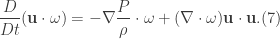
Consider the total derivative of  :
:

where I have used the product rule for derivatives. Also I denote a total derivative as  so as not to confuse it with the notation for an ordinary derivative. Recall the Navier-Stokes’ equation and the vorticity equation

and

Let  and let
  and
and  . Then,

and

If we substitute Eqs. (5) and (6) into Eq.(2), we get
Evaluating each scalar product gives
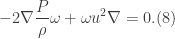
If we divide by 2 and note the definition of the scalar product, we may rewrite this as follows

With this in mind, consider now the total derivative of  multiplied by a volume element
  given by

When the above equation is integrated over a volume  , the total derivative becomes an ordinary time derivative. Thus, Eq.(10) becomes
![\displaystyle \int_{V_{\omega}}\frac{d}{dt}(\textbf{u}\cdot \omega)dV=\iint_{S_{\omega}}\bigg\{\nabla \cdot [-\frac{P}{\rho}\omega + \frac{u^{2}}{2}\omega ]\bigg\}\cdot d\textbf{S}=0. (11)](https://s0.wp.com/latex.php?latex=%5Cdisplaystyle+%5Cint_%7BV_%7B%5Comega%7D%7D%5Cfrac%7Bd%7D%7Bdt%7D%28%5Ctextbf%7Bu%7D%5Ccdot+%5Comega%29dV%3D%5Ciint_%7BS_%7B%5Comega%7D%7D%5Cbigg%5C%7B%5Cnabla+%5Ccdot+%5B-%5Cfrac%7BP%7D%7B%5Crho%7D%5Comega+%2B+%5Cfrac%7Bu%5E%7B2%7D%7D%7B2%7D%5Comega+%5D%5Cbigg%5C%7D%5Ccdot+d%5Ctextbf%7BS%7D%3D0.+%2811%29&bg=ffffff&fg=333333&s=0&c=20201002)
Hence, Eq.(11) shows that helicity is an integral invariant. In this analysis, we have assumed that the fluid is inviscid. If one considers two vortex lines (as Davidson does as a mathematical example), one finds that there exists two contributions to the overall helicity, corresponding to an individual vortex line. If one considers the vorticity multiplied by a volume element, one finds that for each line, their value helicity is the same. Thus, because they are the same, we can say that the overall helicity remains invariant and hence are linked. If they weren’t linked, then the helicity would be 0. In regards to magnetic helicity we define this as

where  is the magnetic vector potential which is described by the following relations

and
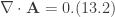
Again, we see that magnetic helicity is also conserved. However, this conservation arises by means of Alfven’s theorem of flux freezing in which the magnetic field lines manage to preserve their topology.


 :
: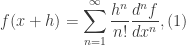

 . Therefore, if we consider the following differences…
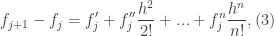


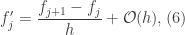
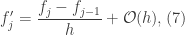
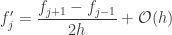
 represents the quadratic, cubic, quartic,quintic,etc. terms. One can use similar logic to derive the second-order finite-difference equations.
