December 2017 – Understanding Physics and Astronomy

Basics of Tensor Calculus and General Relativity-Vectors and Introduction to Tensors (Part I: Vectors)

SOURCE FOR CONTENT: Neuenschwander D.E.,2015. Tensor Calculus for Physics. Johns Hopkins University Press.

At some level, we all are aware of scalars and vectors, but typically we don’t think of aspects of everyday experience as being a scalar or a vector. A scalar is something that has only magnitude, that is it only has a numeric value. A typical example of a scalar would be temperature. A vector, on the other hand, is something that has both a magnitude and direction. This could be something as simple as displacement. If we wish to move a certain distance with respect to our current location we must specify how far to go and in which direction to move. Other examples, (and there are a lot of them), including velocity, force, momentum, etc. Now, tensors are something else entirely. In Neuenschwander’s “Tensor Calculus for Physics”, he recites the rather unsatisfying definition of a tensor as being

” ‘A set of quantities $T_{s}^{r}$ associated with a point P are said to be components of a second-order tensor if, under a change of coordinates, from a set of coordinates $x^{s}$ to $x^{\prime s}$ , they transform according to

$\displaystyle T^{\prime r}_{s}=\frac{\partial x^{\prime r}}{\partial x^{i}}\frac{\partial x^{j}}{\partial x^{\prime s}}T_{j}^{i}. (1)$

where the derivatives are evaluated at the aforementioned point.’ “

Neuenschwander describes his frustration when encountered this so-called definition of a tensor. Like him, I found I had similar frustrations, and as a result, I had even more questions.

We shall start with a discussion of vectors, for an understanding of these quantities are an integral part of tensor analysis.

We define a vector as a quantity that has 3 distinct components and an angle that indicates orientation or direction. There are two types of vectors; those with coordinates and those without. I will be discussing the latter first, but I will consider Neuenschwander’s description in the context of the definition of a vector space. Then I shall move on to the former. Consider a number of arbitrary vectors $\displaystyle \textbf{U}, \textbf{V}, \textbf{W}$ ,etc. If we consider further more and more vectors, we can therefore imagine a space constituted by these vectors; a vector space. To make it formal, here is the definition:

Def. Vector Space:

A vector space $\mathcal{S}$ is the nonempty set of elements (vectors) that satisfy the following axioms

$\displaystyle 1.\textbf{U}+\textbf{V}=\textbf{V}+\textbf{U}; \forall \textbf{U},\textbf{V}\in \mathcal{S},$

$\displaystyle 2. (\textbf{U}+\textbf{V})+\textbf{W}= \textbf{U}+(\textbf{V}+\textbf{W}); \forall \textbf{U},\textbf{V},\textbf{W}\in \mathcal{S},$

$\displaystyle 3. \exists 0 \in \mathcal{S}|\textbf{U}+0=\textbf{U},$

$\displaystyle 4. \forall \textbf{U}\in \mathcal{S}, \exists -\textbf{U}\in \mathcal{S}|\textbf{U}+(-\textbf{U})=0,$

$\displaystyle 5. \alpha(\textbf{U}+\textbf{V})=\alpha\textbf{U}+\alpha\textbf{V}, \forall \alpha \in \mathbb{R}, \forall \textbf{U},\textbf{V}\in \mathcal{S}.$

$\displaystyle 6. (\alpha+\beta) \textbf{U}= \alpha\textbf{U}+\beta\textbf{U}, \forall \alpha,\beta \in \mathbb{R},$

$\displaystyle 7. (\alpha\beta)\textbf{U}= \alpha(\beta\textbf{U}), \forall \alpha,\beta \in \mathbb{R},$

$\displaystyle 8. 1\textbf{U}=\textbf{U}, \forall \textbf{U}\in \mathcal{S},$

and satisfies the following closure properties:

1. If $\textbf{U}\in \mathcal{S}$ , and $\alpha$ is a scalar, then $\alpha\textbf{U}\in \mathcal{S}$ .

2. If $\textbf{U},\textbf{V}\in \mathcal{S}$ , then $\textbf{U}+\textbf{V}\in \mathcal{S}$ .

The first closure property ensures closure under scalar multiplication while the second ensures closure under addition.

In rectangular coordinates, our arbitrary vector may be represented by basis vectors $\hat{i}, \hat{j},\hat{k}$ in the following manner

$\displaystyle \textbf{U}=u\hat{i}+v\hat{j}+w\hat{k}, (1)$

where the basis vectors have the properties

$\displaystyle \hat{i}\cdot \hat{i}=\hat{j}\cdot \hat{j}=\hat{k}\cdot \hat{k}=1, (2.1)$

$\displaystyle \hat{i}\cdot \hat{j}=\hat{j}\cdot \hat{k}=\hat{i}\cdot \hat{k}=0.(2.2)$

The latter of which implies that these basis vectors are mutually orthogonal. We can therefore write these in a more succinct way via

$\displaystyle \hat{e}_{i}\cdot \hat{e}_{j}=\delta_{ij}, (2.3)$

where $\displaystyle \delta_{ij}$ denotes the Kronecker delta:

$\displaystyle \delta_{ij}=\begin{cases} 1, i=j\\ 0, i \neq j \end{cases}. (2.4)$

We may redefine the scalar product by the following argument given in Neuenschwander

$\displaystyle \textbf{U}\cdot \textbf{V}=\sum_{i,j=1}^{3}(U^{i} \hat{e}_{i}) \cdot (V^{j} \hat{e}_{j})=\sum_{i,j=1}^{3}U^{i}V^{j}(\delta_{ij})=\sum_{l=1}^{3}U^{l}V^{l}. (3)$

Similarly we may define the cross product to be

$\displaystyle \textbf{U}\times \textbf{V}=\det\begin{pmatrix} \hat{i} & \hat{j} & \hat{k} \\ U^{x} & U^{y} & U^{z} \\ V^{x} & V^{y} & V^{z} \end{pmatrix}, (4)$

whose $i$ -th component is

$\displaystyle (\textbf{U}\times \textbf{V})^{i}=\textbf{U}\times \textbf{V}=\sum_{i,j=1}^{3}\epsilon^{ijk}U^{j}V^{k}, (5)$

where $\epsilon^{ijk}$ denotes the Levi-Civita symbol. If these indices form an odd permutation $\epsilon^{ijk}=-1$ , if the indices form an even permutation $\epsilon^{ijk}=+1$ , and if any of these indices are equal $\epsilon^{ijk}=0$ .

As a final point, we may relate vectors to relativity by means of defining the four-vector. If we consider the four coordinates $x,y,z,t$ , they collectively describe what is referred to as an event. Formally, an event in spacetime is described by three spatial coordinates and one time coordinate. We may replace these coordinates by $x^{\mu}$ , where $\mu \in \mathbb{Z}^{\pm}$ in which I am defining $\mathbb{Z}^{\pm}=\bigg\{x\in \mathbb{Z}|x\geq 0\bigg\}$ . In words, this means that the index $\mu$ is an integer that is greater than or equal to 0.

Furthermore, the quantity $x^{0}$ corresponds to time, $x^{1,2,3}$ correspond to the x,y, and z coordinates respectively. Therefore, $x^{\mu}=(ct,x,y,z)$ is called the four-position.

In the next post, I will complete the discussion on vectors and discuss in more detail the definition of a tensor (following Neuenschwander’s approach). I will also introduce a few examples of tensors that physics students will typically encounter.

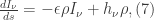
Monte Carlo Simulations of Radiative Transfer: Basics of Radiative Transfer Theory (Part IIa)

SOURCES FOR CONTENT:

Chandrasekhar, S., 1960. “Radiative Transfer”. Dover. 1.
Choudhuri, A.R., 2010. “Astrophysics for Physicists”. Cambridge University Press. 2.
Boyce, W.E., and DiPrima, R.C., 2005. “Elementary Differential Equations”. John Wiley & Sons. 2.1.

Recall from last time , the radiative transfer equation

$\displaystyle \frac{1}{\epsilon \rho}\frac{dI_{\nu}}{ds}= M_{\nu}-N_{\nu}I_{\nu}, (1)$

where $M_{\nu}$ and $N_{\nu}$ are the emission and absorption coefficients, respectively. We can further define the absorption coefficient to be equivalent to $\epsilon \rho$ . Hence,

$\displaystyle N_{\nu}=\frac{d\tau_{\nu}}{ds}, (2)$

which upon rearrangement and substitution in Eq. (1) gives

$\displaystyle \frac{dI_{\nu}(\tau_{\nu})}{d\tau_{\nu}}+I_{\nu}(\tau_{\nu})= U_{\nu}(\tau_{\nu}). (3)$

We may solve this equation by using the method of integrating factors, by which we multiply Eq.(3) by some unknown function (the integrating factor) $\mu(\tau_{\nu})$ yielding

$\displaystyle \mu(\tau_{\nu})\frac{dI_{\nu}(\tau_{\nu})}{d\tau_{\nu}}+\mu(\tau_{\nu})I_{\nu}(\tau_{\nu})=\mu(\tau_{\nu})U_{\nu}(\tau_{\nu}). (4)$

Upon examining Eq.(4), we see that the left hand side is the product rule. It follows that

$\displaystyle \frac{d}{d\tau_{\nu}}\bigg\{\mu(\tau_{\nu})I_{\nu}(\tau_{\nu})\bigg\}=\mu({\tau_{\nu}})U_{\nu}(\tau_{\nu}). (5)$

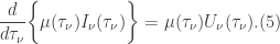
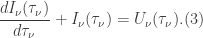
This only works if $d(\mu(\tau_{\nu}))/d\tau_{\nu}=\mu(\tau_{\nu})$ . To show that this is valid, consider the equation for $\mu(\tau_{\nu})$ only:

$\displaystyle \frac{d\mu(\tau_{\nu})}{d\tau_{\nu}}=\mu(\tau_{\nu}). (6.1)$

This is a separable ordinary differential equation so we can rearrange and integrate to get

$\displaystyle \int \frac{d\mu(\tau_{\nu})}{\mu(\tau_{\nu})}=\int d\tau_{\nu}\implies \ln(\mu(\tau_{\nu}))= \tau_{\nu}+C, (6.2)$

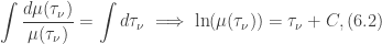
where $C$ is some constant of integration. Let us assume that the constant of integration is $0$ , and let us also take the exponential of (6.2). This gives us

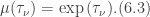
$\displaystyle \mu(\tau_{\nu})=\exp{(\tau_{\nu})}. (6.3)$

This is our integrating factor. Just as a check, let us take the derivative of our integrating factor with respect to $d\tau_{\nu}$ ,

$\displaystyle \frac{d}{d\tau_{\nu}}\exp{(\tau_{\nu})}=\exp{(\tau_{\nu})},$

Thus this requirement is satisfied. If we now return to Eq.(4) and substitute in our integrating factor we get

$\displaystyle \frac{d}{d\tau_{\nu}}\bigg\{\exp{(\tau_{\nu})}I_{\nu}(\tau_{\nu})\bigg\}=\exp{(\tau_{\nu})}U_{\nu}(\tau_{\nu}). (7)$

We can treat this as a separable differential equation so we can integrate immediately. However, we are integrating from an optical depth $0$ to some optical depth $\tau_{\nu}$ , hence we have that

$\displaystyle \int_{0}^{\tau_{\nu}}d\bigg\{\exp{(\tau_{\nu})}I_{\nu}(\tau_{\nu})\bigg\}=\int_{0}^{\tau_{\nu}}\bigg\{\exp{(\bar{\tau}_{\nu})}U_{\nu}(\bar{\tau}_{\nu})\bigg\}d\bar{\tau}_{\nu}, (8)$

We find that

$\displaystyle \exp{(\tau_{\nu})}I_{\nu}(\tau_{\nu})-I_{\nu}(0)=\int_{0}^{\tau_{\nu}}\bigg\{\exp{(\bar{\tau}_{\nu})}U_{\nu}(\bar{\tau}_{\nu})\bigg\}d\bar{\tau}_{\nu} (9),$

where if we add $I_{\nu}(0)$ and divide by $\exp{(\tau_{\nu})}$ we arrive at the general solution of the radiative transfer equation

$\displaystyle I_{\nu}(\tau_{\nu}) = I_{\nu}(0)\exp{(-\tau_{\nu})}+\int_{0}^{\tau_{\nu}}\exp{(\bar{\tau}_{\nu}-\tau_{\nu})}U_{\nu}(\bar{\tau}_{\nu})d\bar{\tau}_{\nu}. (10)$

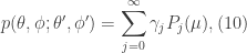
This is the mathematically formal solution to the radiative transfer equation. While mathematically sound, much of the more interesting physical phenomena require more complicated equations and therefore more sophisticated methods of solving them (an example would be the use of quadrature formulae or $n$ -th approximation for isotropic scattering).

Recall also that in general we can write the phase function $p(\theta,\phi; \theta^{\prime},\phi^{\prime})$ via the following

$\displaystyle p(\theta,\phi;\theta^{\prime},\phi^{\prime})=\sum_{l=0}^{\infty}\gamma_{l}P_{l}(\cos{\Theta}). (11)$

Let us consider the case for which $l=0$ in the sum given by (11). This then would mean that the phase function is constant

$p(\theta,\phi;\theta^{\prime},\phi^{\prime})=\gamma_{0}=const. (12)$

Such a phase function is consistent with isotropic scattering. The term isotropic means, in this context, that radiation scattered is the same in all directions. Such a case yields a source function of the form

$\displaystyle U_{\nu}(\tau_{\nu})=\frac{1}{4\pi}\int_{0}^{\pi}\int_{0}^{2\pi}\gamma_{0}I_{\nu}(\tau_{\nu})\sin{\theta^{\prime}}d\theta^{\prime}d\phi^{\prime}, (13)$

where upon use in the radiative transfer equation we get the integro-differential equation

$\displaystyle \frac{dI_{\nu}(\tau_{\nu})}{d\tau_{\nu}}+I_{\nu}(\tau_{\nu})= \frac{1}{4\pi}\int_{0}^{\pi}\int_{0}^{2\pi}\gamma_{0}I_{\nu}(\tau_{\nu})\sin{\theta^{\prime}}d\theta^{\prime}d\phi^{\prime}. (14)$

Solution of this equation is beyond the scope of the project. In the next post I will discuss Rayleigh scattering and the corresponding phase function.

Elementary Methods to Solving Integral Equations: Overview of Series

After taking a differential equations course, I reasoned that if there are differential equations, then there must be an “inverse theory” of integral equations. I was able to find a text that discussed the basics, but interestingly videos discussing this topic were scarce. So I thought I would do a (short) series on some basic methods towards solving these types of equations and perhaps apply them to a physical problem.

This series will discuss two types of integral equations:

Fredholm Equations

Volterra Equations

I will also discuss…

Symmetric Kernels and Orthogonal Systems of Functions.

Note & Status:

This series is meant to be a shorter, supplementary series. My main focus right now is the Monte Carlo Simulations of Radiative Transfer series and once that is finished, I will move on to the Basics of Tensor Calculus series. I am doing this series on integral equations out of pure mathematical curiosity. I should have a couple of new posts up in the next few days.

Basics of Tensor Calculus and General Relativity: Overview of Series

Of the many topics that I have studied in the past, one of the most confusing topics that I have encountered is the concept of a tensor. Every time that I heard the term tensor, it was mentioned for the sake of mentioning it and my professors would move on. Others simply ignored the existence of tensors, but every time they were brought up I was intrigued. So the purpose of this series is to attempt to discover how tensors work and how they relate to our understanding of the universe, specifically in the context of general relativity.

The text I will be following for this will be Dwight E. Neuenschwander’s “Tensor Calculus for Physics”. I will be documenting my interpretation of the theory discussed in this text, and I will use the text “General Relativity: An Introduction for Physicists” by M.P. Hobson, G. Efstathiou, and A.N. Lasenby to discuss the concepts developed in the context of general relativity. I will list the corresponding chapter titles associated with each post.

Here is an approximate agenda (note that this will take some time as I am learning this as I post, so posts in this series may be irregular).

Post I: Tensor Calculus: Introduction and Vectors

Post II: Tensor Calculus: Vector Calculus and Coordinate Transformations

Post III: General Relativity: Basics of Manifolds and Coordinates

Post IV: General Relativity: Vector Calculus on Manifolds

Post V: Tensor Calculus: Introduction to Tensors and the Metric Tensor

Post VI: Tensor Calculus: Derivatives of Tensors

Post VII: General Relativity: Tensor Calculus on Manifolds

Post VIII: Tensor Calculus: Curvature

Post IX: General Relativity: Equivalence Principle and Spacetime Curvature

Post X: General Relativity: The Gravitational Field Equations

The series will end with the Einstein field equations (EFEs) since they are the crux of the general theory of relativity. The posts in this series will come in their own time as they can be quite difficult and time-consuming, but I will do my best to understand it. I welcome any feedback you may have, but please be respectful.

Monte Carlo Simulations of Radiative Transfer: Basics of Radiative Transfer Theory (Part I)

SOURCE FOR CONTENT: Chandrasekhar, S., 1960. Radiative Transfer. 1.

In this post, I will be discussing the basics of radiative transfer theory necessary to understand the methods used in this project. I will start with some definitions, then I will look at the radiative transfer equation and consider two simple cases of scattering.

The first definition we require is the specific intensity, which is the amount of energy associated with a specific frequency $dE_{\nu}$ passing through an area $dA$ constrained to a solid angle $d\Omega$ in a time $dt$ . We may write this mathematically as

$dE_{\nu}=I_{\nu}\cos{\theta}d\nu d\Sigma d\Omega dt. (1)$

We must also consider the net flux given by

$\displaystyle d\nu d\Sigma dt \int I_{\nu}\cos{\theta}d\Omega, (2)$

where if we integrate over all solid angles $\Omega$ we get

$\pi F_{\nu}=\displaystyle \int I_{\nu}\cos{\theta}d\Omega. (3)$

Let $d\Lambda$ be an element of the surface $\Lambda$ in a volume $V$ through which radiation passes. Further let $\Theta$ and $\theta$ denote the angles which form normals with respect to elements $d\Lambda$ and $d\Sigma$ . These surfaces are joined by these normals and hence we have the surface across which energy flows includes the elements $d\Lambda$ and $d\Sigma$ , given by the following:

$I_{\nu}\cos{\Theta}d\Sigma d\Omega^{\prime}d\nu = I_{\nu}d\nu \frac{\cos{\Theta}\cos{\theta}d\Sigma d\Lambda}{r^{2}} (4),$

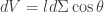
where $d\Omega^{\prime}=d\Lambda \cos{\Theta}/r^{2}$ is the solid angle subtended by the surface element $d\Lambda$ at a point $P$ and volume element $dV=ld\Sigma \cos{\theta}$ is the volume that is intercepted in volume $V$ . If we take this further, and integrate over all $V$ and $\Omega$ we arrive at

$\displaystyle \frac{d\nu}{c}\int dV \int I_{\nu} d\Omega=\frac{V}{c}d\nu \int I_{\nu}d\Omega, (5)$

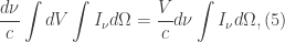
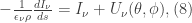
where if the radiation travels some distance $L$ in the volume, then we must multiply Eq.(5) by $l/c$ , where $c$ is the speed of light.

We now define the integrated energy density as being

$U_{\nu}=\displaystyle \frac{1}{c}\int I_{\nu}d\Omega, (6.1)$

while the average intensity is

$J_{\nu}=\displaystyle \frac{1}{4\pi}\int I_{\nu}d\nu, (6.2)$

and the relation between these two equations is

$U_{\nu}=\frac{4\pi}{c}J_{\nu}. (6.3)$

I will now introduce the radiative transfer equation. This equation is a balance between the amount of radiation absorbed and the radiation that is emitted. The equation is,

$\frac{dI_{\nu}}{ds}=-\epsilon \rho I_{\nu}+h_{\nu}\rho, (7)$

where if we divide by $\epsilon \rho$ we get

$-\frac{1}{\epsilon_{\nu}\rho}\frac{dI_{\nu}}{ds}=I_{\nu}+U_{\nu}(\theta, \phi), (8)$

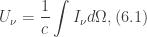
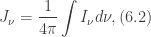
where $U(\theta,\phi)$ represents the source function given by

$U_{\nu}(\theta,\phi)=\displaystyle \frac{1}{4\pi}\int_{0}^{\pi}\int_{0}^{2\pi}p(\theta,\phi;\theta^{\prime},\phi^{\prime})I_{\nu}\sin{\theta^{\prime}}d\theta^{\prime}d\phi^{\prime}. (9)$

The source function is typically the ratio between the absorption and emission coefficients. One of the terms in the source function is the phase function which varies according to the specific scattering geometry. In its most general form, we can represent the phase function as an expansion of Legendre polynomials:

$p(\theta, \phi; \theta^{\prime},\phi^{\prime})=\displaystyle \sum_{j=0}^{\infty}\gamma_{j}P_{j}(\mu), (10)$

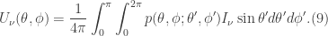
where we have let $\mu = \cos{\theta}$ (in keeping with our notation in previous posts).

In Part II, we will discuss a few simple cases of scattering and their corresponding phase functions, as well as obtaining the formal solution of the radiative transfer equation. (DISCLAIMER: While this solution will be consistent in a mathematical sense, it is not exactly an insightful solution since much of the more interesting and complex cases involve the solution of either integro-differential equations or pure integral equations (a possible new topic).)

Simple Harmonic Oscillators (SHOs) (Part I)

We all experience or see this happening in our everyday experience: objects moving back and forth. In physics, these objects are called simple harmonic oscillators. While I was taking my undergraduate physics course, one of my favorite topics was SHOs because of the way the mathematics and physics work in tandem to explain something we see everyday. The purpose of this post is to engage followers to get them to think about this phenomenon in a more critical manner.

Every object has a position at which these objects tend to remain at rest, and if they are subjected to some perturbation, that object will oscillate about this equilibrium point until they resume their state of rest. If we pull or push an object with an applied force $F_{A}$ we find that this force is proportional to Hooke’s law of elasticity, that is, $F_{A}=-k\textbf{r}$ . If we consider other forces we also find that there exists a force balance between the restoring force (our applied force), a resistance force, and a forcing function, which we assume to have the form

$F=F_{forcing}+F_{A}-F_{R}= -k\textbf{r}-\beta \dot{\textbf{r}}; (1)$

note that we are assuming that the resistance force is proportional to the speed of an object. Suppose further that we are inducing these oscillations in a periodic manner by given by

$F_{forcing}=F_{0}\cos{\omega t}. (2)$

Now, to be more precise, we really should define the position vector. So, $\textbf{r}=x\hat{i}+y\hat{j}+z\hat{k}$ . Therefore, we actually have a system of three second order linear non-homogeneous ordinary differential equations in three variables:

$m\ddot{ x}+\beta \dot{x}+kx=F_{0}\cos{\omega t}, (3.1)$

$m\ddot{y}+\beta \dot{y}+ky=F_{0}\cos{\omega t}, (3.2)$

$m\ddot{z}+\beta \dot{z}+kz=F_{0}\cos{\omega t}. (3.3)$

(QUICK NOTE: In the above equations, I am using the Newtonian notation for derivatives, only for convenience.) I will just make some simplifications. I will divide both sides by the mass, and I will define the following parameters: $\gamma \equiv \beta/m$ , $\omega_{0} \equiv k/m$ , and $\alpha \equiv F_{0}/m$ . Furthermore, I am only going to consider the $y$ component of this system. Thus, the equation that we seek to solve is

$\ddot{y}+\gamma \dot{y}+\omega_{0}y=\alpha\cos{\omega t}. (4)$

Now, in order to solve this non-homogeneous equation, we use the method of undetermined coefficients. By this we mean to say that the general solution to the non-homogeneous equation is of the form

$y = Ay_{1}(t)+By_{2}(t)+Y(t), (5)$

where $Y(t)$ is the particular solution to the non-homogeneous equation and the other two terms are the fundamental solutions of the homogeneous equation:

$\ddot{y}_{h}+\gamma \dot{y}_{h}+\omega_{0} y_{h} = 0. (6)$

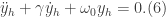
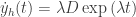
Let $y_{h}(t)=D\exp{(\lambda t)}$ . Taking the first and second time derivatives, we get $\dot{y}_{h}(t)=\lambda D\exp{(\lambda t)}$ and $\ddot{y}_{h}(t)=\lambda^{2}D\exp{(\lambda t)}$ . Therefore, Eq. (6) becomes, after factoring out the exponential term,

$D\exp{(\lambda t)}[\lambda^{2}+\gamma \lambda +\omega_{0}]=0. (7)$

Since $D\exp{(\lambda t)}\neq 0$ , it follows that

$\lambda^{2}+\gamma \lambda +\omega_{0}=0. (8)$

This is just a disguised form of a quadratic equation whose solution is obtained by the quadratic formula:

$\lambda =\frac{-\gamma \pm \sqrt[]{\gamma^{2}-4\omega_{0}}}{2}. (9)$

Part II of this post will discuss the three distinct cases for which the discriminant $\sqrt[]{\gamma^{2}-4\omega_{0}}$ is greater than, equal to , or less than 0, and the consequent solutions. I will also obtain the solution to the non-homogeneous equation in that post as well.

Monte Carlo Simulations of Radiative Transfer: Project Overview

The goal of this project was to simulate radiative transfer in the circumbinary disk GG Tau by using statistical methods (i.e. Monte Carlo methods). To provide some context for the project, I will describe the astrophysical system that I considered, and I will describe the objectives of the project

Of the many stars in the night sky, a significant number of them, when you are able to resolve them, are in fact binary stars. These are star systems in which two stars orbit a common center of mass known as a barycenter. For this reason, we regard GG Tau to be a close binary system; a system in which two stars are separated by a significant distance comparable to the diameters of each star.

The system of GG Tau has four known components with a hypothesized fifth component. There is a disk of material encircling the entire system which we call a circumbinary disk. Additionally, there is also an inner disk of material that surrounds the primary and secondary components referred to as a circumstellar disk.

The goal of this project was to use Monte Carlo methods to simulate radiative transfer processes present in GG Tau. This is accomplished through the use of importance sampling two essential quantities over cumulative distribution function of the form

$\displaystyle \xi=\int_{0}^{L} \mathcal{P}(x)dx\equiv \psi(x_{0}), (1)$

using FORTRAN code. I will discuss the mathematical background of probability and Monte Carlo methods (stochastic processes) in more detail in a later post. The general process of radiative transfer is relatively simple. Starting with an emitter, radiation travels from its emission point, travels a certain distance, and at this point the radiation could either be scattered into an angle different from the incidence angle, or it can be absorbed by the material. In the context of this project, the emitter (or emitters) are the primary and secondary components of GG Tau. The radiation emitted is electromagnetic radiation, or light. This light will travel a distance $L$ after which the light is either scattered or absorbed. The code uses Eq.(1) (cumulative distribution function) to sample optical depths and scattering angles to calculate the distance traveled $L$ . I will reserve the exact algorithm for a future post as well. In the next post, I will discuss the basics of radiative transfer theory as presented in the text “Radiative Transfer” by S. Chandrasekhar, 1960.

The following are the sources used in this project

Wood, K., Whitney, B., Bjorkman, J., and Wolff M., 2013. Introduction to Monte Carlo Radiative Transfer.

Whitney, B. A., 2011. Monte Carlo Radiative Transfer. Bull. Astr. Soc. India.

Kitamura, Y., Kawabe, R., Omodaka, T., Ishiguro, M., and Miyama, S., 1994. Rotating Protoplanetary Gas Disk in GG Tau. ASP Conference Series. Vol. 59.

Piètu, V., Gueth, F., Hily-Blant, P., Schuster, K.F., and Pety, J., 2011. High Resolution Imaging of the GG Tauri system at 267 GHz. Astronomy & Astrophysics. 528. A81.

Skrutskie, M.F., Snell, R.L., Strom, K.M., Strom, S.E., and Edwards, S., 1993. Detection of Circumstellar Gas Associated with GG Tauri. The Astrophysical Journal. 409:422-428.

Choudhuri, A.R., 2010. Astrophysics for Physicists. 2.

Carroll B.W., Ostlie, D.A., 2007. An Introduction to Modern Astrophysics. 9,10.

Chandrasekhar, S., 1960. Radiative Transfer. 1.

Schroeder, D., 2000. Introduction to Thermal Physics. 8.

Ross, S., 2010. Introduction to Probability Model. 2,4,11.

I obtained the FORTRAN code from K. Wood via the following link. (For the sake of completeness the URL is: www-star.st-and.ac.uk/~kw25/research/montecarlo/montecarlo.html)

Share this:

Share this:

Share this:

Share this:

Share this:

Share this:

Share this: