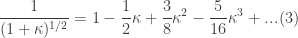
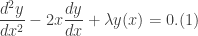
Some time ago, I wrote a post discussing the solution to Legendre’s ODE. In that post, I discussed what is an alternative definition of Legendre polynomials in which I stated Rodriguez’s formula:

where
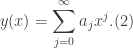
 ,
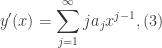
,
and
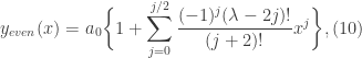
in which I have let  and
and  corresponding to the even and odd expressions for the Legendre polynomials.
However, in this post I shall be using the approach of the generating function. This will be from a purely mathematical perspective, so I am not applying this to any particular topic of physics.
Consider a triangle with sides  and angles
  . The law of cosines therefore maintains that

We can factor out  from the left hand side of Eq.(1), take the square root and invert this yielding

Now, we can expand this by means of the binomial expansion. Let  , therefore the binomial expansion is
Hence if we expand this in terms of the sides and angle(s) of the triangle and group by powers of  we get

Notice the coefficients, these are precisely the expressions for the Legendre polynomials. Therefore, we see that
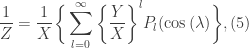
or
![\displaystyle \frac{1}{Z}=\frac{1}{\sqrt[]{X^{2}+Y^{2}-2XY\cos{(\lambda)}}}=\sum_{l=0}^{\infty}\frac{Y^{l}}{X^{l+1}}P_{l}(\cos{(\lambda)}. (6)](https://s0.wp.com/latex.php?latex=%5Cdisplaystyle+%5Cfrac%7B1%7D%7BZ%7D%3D%5Cfrac%7B1%7D%7B%5Csqrt%5B%5D%7BX%5E%7B2%7D%2BY%5E%7B2%7D-2XY%5Ccos%7B%28%5Clambda%29%7D%7D%7D%3D%5Csum_%7Bl%3D0%7D%5E%7B%5Cinfty%7D%5Cfrac%7BY%5E%7Bl%7D%7D%7BX%5E%7Bl%2B1%7D%7DP_%7Bl%7D%28%5Ccos%7B%28%5Clambda%29%7D.+%286%29&bg=ffffff&fg=333333&s=0&c=20201002)
Thus we see that the generating function  generates the Legendre polynomials. Two prominent uses of these polynomials includes gravity and its application to the theory of potentials of a spherical mass distributions, and the other is that of electrostatics. For example, suppose we have the potential equation

We may use the result of the generating function to get the following result for the electric potential due an arbitrary charge distribution
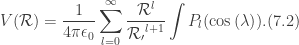
(For more details, see Chapter 3 of Griffith’s text: Introduction to Electrodynamics.)


![\displaystyle \sum_{j=0}^{\infty}[(j+2)(j+1)a_{j+2}-2ja_{j}+\lambda a_{j}]x^{j}=0. (7)](https://s0.wp.com/latex.php?latex=%5Cdisplaystyle+%5Csum_%7Bj%3D0%7D%5E%7B%5Cinfty%7D%5B%28j%2B2%29%28j%2B1%29a_%7Bj%2B2%7D-2ja_%7Bj%7D%2B%5Clambda+a_%7Bj%7D%5Dx%5E%7Bj%7D%3D0.+%287%29&bg=ffffff&fg=333333&s=0&c=20201002)