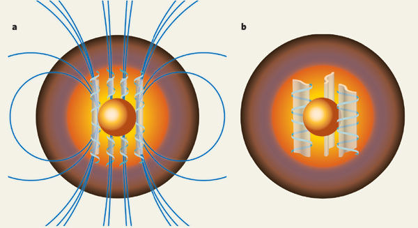
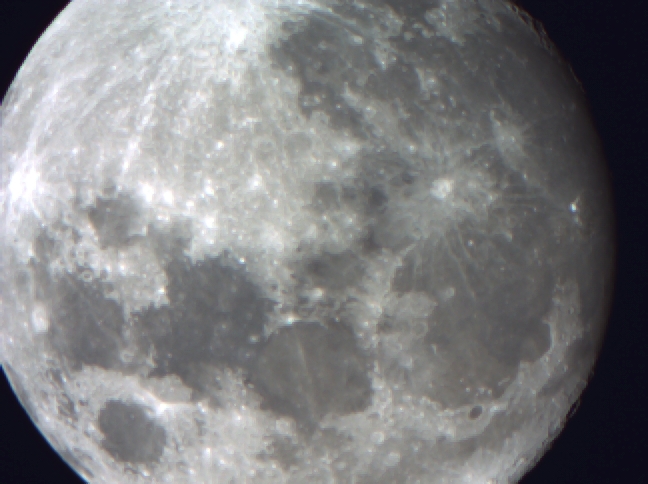
FEATURED IMAGE CREDIT: U.R. Christensen from the Nature article: “Earth Science: A Sheet-Metal Dynamo”
The image shows the overall distortion of magnetic field lines inside the core and its’ effect on the magnetic field outside.
This post shall continue to derive the principal equations of ideal one-fluid magnetohydrodynamics. Here I shall derive the continuity equation and the vorticity equation. Furthermore, I shall show that the Boussinesq approximation results in a zero-valued divergence. I have consulted the following works while researching this topic:
Davidson, P.A., 2001. An Introduction to Magnetohydrodynamics. 3-4,6.
Murphy, N., 2016. Ideal Magnetohydrodynamics. Lecture presentation. Harvard-Smithsonian Center for Astrophysics.
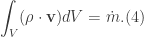
Consider a fluid element through which fluid passes. The mass of this element can be represented as the volume integral of the material density 

Take the first order time derivative of the mass, we arrive at

We now make a slight notation change; let the triple integral be represented as

Now, the mass flux through a surface element 

We may write this as

Now, we invoke Gauss’s theorem (also known as the Divergence Theorem) of the form

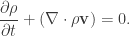
we get

Since the integral cannot be zero, the integrand must be. Therefore, we get the continuity equation:

Recall the following equation from a previous post (specifically Eq. (6) of that post)
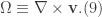
Now we define the concept of vorticity. Conceptually, this refers to the rotation of the fluid within its velocity field. Mathematically, we define the vorticity 
Now recall, the vector identity
which upon rearrangement is
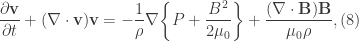
Using Eq.(10.2) with Eq.(8) we get
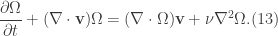
Recall our definition of vorticity. Upon taking the curl of Eq.(11) we arrive at a variation of the induction equation (see post)
Next, we invoke another vector identity

Using Eq. (12.2) in Eq. (12.1) yields the vorticity equation
Returning to the continuity equation:
I will now show that the flow does not diverge. In other words, there are no sources in the fluid velocity field. The Boussinesq approximation’s main assertion is that of isopycnal flow (i.e. flow of constant density). Therefore, let 
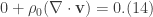
The temporal derivative is a derivative of a non-zero constant which is itself zero. This just leaves 

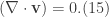
Hence, the divergence of the fluid’s velocity field is zero.

 . Furthermore, by the method of separation of variables we suppose that the solution is a product of eigenfunctions of the form
  . Hence, Laplace’s equation becomes
 into
into  . Rewriting (2) and multiplying by
 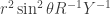 , we get
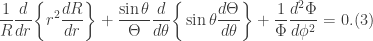
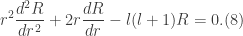
 , yielding

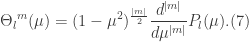
 and carry out the derivative in the angular component to get the Associated Legendre equation:
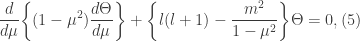
 . The solutions to this equation are known as the associated Legendre functions. However, instead of solving this difficult equation by brute force methods (i.e. power series method), we consider the case for which
  . In this case, Eq.(5) simplifies to Legendre’s differential equation discussed
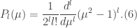
 and for complex solutions
  , thus we can write the solutions as series whose indices run from 0 to l for the real-values and from -l to l for the complex-valued solutions.
 in place of the angular component, we get
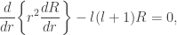

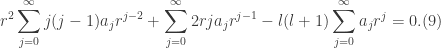
![\displaystyle \sum_{j=0}^{\infty}[j(j-1)+2j-l(l+1)]a_{j}r^{j}=0.](https://s0.wp.com/latex.php?latex=%5Cdisplaystyle+%5Csum_%7Bj%3D0%7D%5E%7B%5Cinfty%7D%5Bj%28j-1%29%2B2j-l%28l%2B1%29%5Da_%7Bj%7Dr%5E%7Bj%7D%3D0.&bg=ffffff&fg=333333&s=0&c=20201002)
 , this means that

 , we arrive at
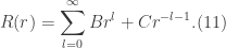
![\displaystyle \psi(r,\theta,\phi) = \sum_{l=0}^{\infty} \sum_{m=0}^{\infty}[Br^{l}+Cr^{-l-1}]\Theta_{l}^{m}(\mu)A\exp({im\phi}), (12)](https://s0.wp.com/latex.php?latex=%5Cdisplaystyle+%5Cpsi%28r%2C%5Ctheta%2C%5Cphi%29+%3D+%5Csum_%7Bl%3D0%7D%5E%7B%5Cinfty%7D+%5Csum_%7Bm%3D0%7D%5E%7B%5Cinfty%7D%5BBr%5E%7Bl%7D%2BCr%5E%7B-l-1%7D%5D%5CTheta_%7Bl%7D%5E%7Bm%7D%28%5Cmu%29A%5Cexp%28%7Bim%5Cphi%7D%29%2C%C2%A0+%2812%29&bg=ffffff&fg=333333&s=0&c=20201002)
![\displaystyle \psi(r,\theta,\phi)=\sum_{l=0}^{\infty}\sum_{m=-l}^{l}[Br^{l}+Cr^{-l-1}]\Theta_{l}^{m}(\mu)A\exp({im\phi}), (13)](https://s0.wp.com/latex.php?latex=%5Cdisplaystyle+%5Cpsi%28r%2C%5Ctheta%2C%5Cphi%29%3D%5Csum_%7Bl%3D0%7D%5E%7B%5Cinfty%7D%5Csum_%7Bm%3D-l%7D%5E%7Bl%7D%5BBr%5E%7Bl%7D%2BCr%5E%7B-l-1%7D%5D%5CTheta_%7Bl%7D%5E%7Bm%7D%28%5Cmu%29A%5Cexp%28%7Bim%5Cphi%7D%29%2C+%2813%29&bg=ffffff&fg=333333&s=0&c=20201002)
