
IMAGE CREDIT: NASA/JPL
SOURCE FOR CONTENT: Classical Dynamics of Particles and Systems. Thornton and Marion. 5th Edition.
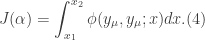
Consider a functional

where 

Additionally, we will find it useful to define

Further we may also define an integral functional by way of integrating Eq.(1) over the interval 

Two necessary conditions that are used to derive the Euler-Lagrange equation include

and

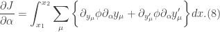
Let us take the derivative of 

Carrying out the derivative operator on the right-hand-side of Eq.(7) we get
From Eqs.(2) and (3) we see that

and

Thus Eq.(8) becomes…

Consider the second term under the summation. We may make use of integration by parts to obtain the following

By the necessary condition (Eq.(5)), it follows that

Additionally, in Eq.(13) above, we have also made use of the condition that 

Update: the next posts will be those discussed on my Facebook page. Namely, I intend to continue with my Research Series and my series in Tensor Calculus and General Relativity with various ancillary posts in my Astrophysics Series.
Clear Skies!

 and the orbital radius vector of Alpha Centauri B is
  . The masses of Alpha Centauri A and B are
  , and
, and  , respectively. The total mass of the binary orbit
  is the sum of the individual masses of each component. In the context of this system, we encounter what is called the two-body problem of which there exists a special case known as the Kepler Problem (by the way let me know if that would be something that you guys would want to see…). We can simplify this two-body problem by making use of center-of-mass coordinates wherein we define the reduced mass
  . Therefore, the derivation of the total energy of the binary system of Alpha Centauri A and B will be carried out in such a coordinate system.


 represents the separation distance between the two components. Let us take the derivative of Eqs.(0.1) and (0.2) to get


 in Eq.(0.3) we get the total energy of the binary Alpha Centauri A and B. This is true for any binary system assuming center-of-mass coordinates.