June 2018 – Understanding Physics and Astronomy

While I was in school, one of my professors set this problem to me and my classmates and challenged us to solve it over the next few days. I found the challenge intriguing and it fascinated me, so I thought it was worth sharing. The problem was this:

Show that

$\displaystyle v(x,t) = \int_{-\infty}^{\infty} f(x-y,t)g(y)dy, (1.1)$

where $\displaystyle g(y)$ has finite support and also satisfies the PDE

$\displaystyle \frac{\partial v}{\partial t} = -\kappa \frac{\partial^{2}v}{\partial x^{2}}. (1.2)$

First off, what does finite support mean? Mathematically speaking, a function has support which is characterized by a subset of its domain whose members do not map to zero, and yet are finite. (Just as a quick note: much of the proper definitions require an understanding in mathematical analysis and measure theory, something which I have not studied in detail, so take that explanation with a grain of salt.)

As for the solution, we can rewrite the given PDE as

$\displaystyle \frac{\partial v}{\partial t} - \kappa \frac{\partial^{2}v}{\partial x^{2}} = 0. (2)$

The PDE requires a first-order time derivative and a second-order spatial derivative.

$\displaystyle \therefore \frac{\partial v}{\partial t} = \frac{\partial}{\partial t}\int_{-\infty}^{\infty} f(x-y,t)g(y)dy, (3.1)$

and

$\displaystyle \frac{\partial^{2} v}{\partial x^{2}} = \frac{\partial^{2}}{\partial x^{2}}\int_{-\infty}^{\infty} f(x-y,t)g(y)dy. (3.2)$

Next, we substitute Eqs. (3.1) and (3.2) into Eq.(2), yielding

$\displaystyle \frac{\partial}{\partial t}\int_{-\infty}^{\infty} f(x-y,t)g(y)dy -\kappa \frac{\partial^{2}}{\partial x^{2}}\int_{-\infty}^{\infty} f(x-y,t)g(y)dy = 0. (4)$

Note that taking the derivative of a function and then integrating that function is equivalent to integrating the function and differentiating the same function, in conjunction with the fact that the sum or difference of the integrals is the integral of the sum or difference (proofs of these facts are typically covered in a course in real analysis). Taking advantage of these gives

$\displaystyle \int_{-\infty}^{\infty} \bigg\{\frac{\partial}{\partial t}f(x-y,t)-\kappa\frac{\partial^{2}}{\partial x^{2}}f(x-y,t)\bigg\}g(y)dy = 0. (5)$

Notice that the terms contained in the brackets equate to $\displaystyle 0$ . This means that

$\displaystyle \int_{-\infty}^{\infty} 0 \cdot g(y)dy = 0. (6)$

This implies that the function $\displaystyle v(x,t)$ does satisfy the given PDE (Eq.(2)).

References:

Definition of Support in Mathematics: https://en.wikipedia.org/wiki/Support_(mathematics)

While I was an undergraduate, one of my smaller research projects involved observing the variable star W Ursae Majoris.

In general, there are six types of binary star systems: Optical double, Visual binary, Astrometric binary, Eclipsing binary, Spectrum binary, and Spectroscopic binary.

In this project, my classmate and I were interested in the eclipsing binary (EW) W Ursae Majoris. An eclipsing binary is a binary system in which one of the stars will pass in front of its companion, effectively causing an eclipse. We are able to observe this by way of generating the light curves of the system. An example light curve is shown below:

(Image was obtained at the URL: https://imagine.gsfc.nasa.gov/educators/hera_college/binary-model.html)

The graph shows a plot of intensity over time (which in this case is an orbital period). Observations of an EW should show dips in the intensity of the two stars. What is really fascinating to me is that we can gain valuable information from this graph. For example, the length of a dip can indicate the masses of the star. If we have a star of mass $m_{1}$ and the other is $m_{2}$ such that $m_{2}>m_{1}$ , and if the duration of the decrease in intensity of the system is significant we can then infer that the mass passing in front of its companion is that of $m_{1}$ . By default, the mass that is being “eclipsed” is $m_{2}$ . Conversely, if the intensity decreases but only for a short while, the positions are reversed, with $m_{2}$ passing in front (relatively speaking) and $m_{1}$ is being “eclipsed”. (I am assuming that the barycenter (i.e. the system’s center of mass) is equidistant from the centers of the two stars.)

Another form of classification of binary stars is whether or not the binary system components are touching or not. More precisely, there are three kinds of close binaries: detached, semi-detached, and contact binary. There are sub-categories of contact binaries: near contact, contact, overcontact, and double contact.

An equipotential surface map of a system (assuming that the binary system has a mass ratio of 2:1, which may be incorrect as most W UMa binaries have a mass ratio of 10:1) is shown below:

Image Credit: Fig.1 of Terrell, D., Eclipsing Binary Stars: Past, Present, and Future. JAAVSO Vol. 30, 2001.

To quickly elaborate, each type of contact binary will fill its inner Lagrangian surface (aka Roche lobes) to an extent. In the context of our project, W Ursae Majoris is an overcontact eclipsing binary system. This type of binary will overfill its inner Lagrangian surface. As a result of this, processes such as mass transfer and accretion can occur. The diagram below shows the orbital evolution of a W UMa EW AC Bootis (in addition to being its own binary system, W UMa is also a class of close binaries)

Image Credit: Fig. 15 of Alton, K., A Unified Roche-Model Light Curve Solution for the W UMa Binary AC Bootis. JAAVSO. Vol. 38, 2010.

The objective of the project was to image the eclipsing binary, measure the apparent magnitude, to process the images, and to obtain a light curve. To observe this system, a classmate and I made use of the 20″ Ritchey-Chrétien telescope at the university observatory. We made use of the CCD camera attached and set a sequence of images to be taken every two minutes. W UMa has a period of approximately 8 hours, however, due to time constraints (and as much as I would have liked to, the weather was not conducive for observations exceeding two hours), we ended up only taking images for around two hours.

After the session was over, we ended up taking a total of roughly 40-50 images. Additionally, the software used to capture the images simultaneously measured the magnitude of W UMa at the time each image was taken. This allowed us to use Excel (and later on MATLAB) to obtain a partial light curve. However, since this is a partial light curve, we can say that an eclipse (and a short one at that) occurs, yet we cannot determine whether or not the local minimum depicted in the graph below is a primary or a secondary minimum–we simply do not have enough data.

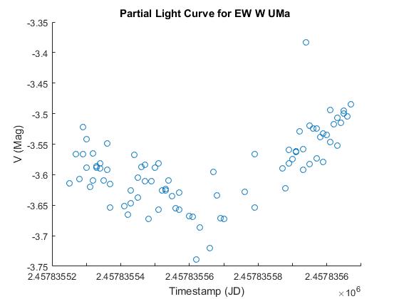
In addition to the partial light curve above, we were able to process the images (using Registax v.6). Below is a stacked image of W UMa. The big blob near the center of the image is the binary. The binary is not able to be resolved by telescopes component-wise.

References:

Caroll, B.W., and Ostlie, D. A., Introduction to Modern Astrophysics. 2017. Cambridge University Press. 7.

Catalog and Atlas of Eclipsing Binaries (CALEB): Types of Binary Stars

http://www.daviddarling.info/encyclopedia/C/close_binary.html

American Association of Variable Star Observers (AAVSO) URL: https://www.aavso.org/vsots_wuma

Journal of American Association of Variable Star Observers: Figure References

Month: June 2018

A Narrow, Technical Problem in Partial Differential Equations

Observing the Variable Star W Ursae Majoris

Share this:

Share this: